Performance, Scalability, and Troubleshooting
Introduction
Our journey begins with a major challenge; the annual "Mega-Sale Monday" event. Our flagship e-commerce website, now partially migrated to VM-based services on OpenShift Virtualization, is anticipating an unprecedented surge in traffic. Last year, our website crashed due to unexpected traffic spikes, leading to significant lost sales and frustrated customers. This year, while we are determined to be prepared, we need to know how to recognize unexpected issues in our environment and how to address them to ensure that the scenario from last year does not repeat itself. In this module you will learn how to discover a high-load scenario on your cluster, how to mitigate and remediate the cluster by scaling resources both vertically and horizontally, and finally learn how to balance the resources on your cluster for future events.
Credentials for the Red Hat OpenShift Console
Your OpenShift cluster console is available here.
Your local admin login is available with the following credentials:
-
User:
username -
Password:
password
You will first see a page that asks you to choose an authentication provider, click on htpasswd_provider.

You will then be presented with a login screen where you can copy/paste your credentials.

Enable and Explore Alerts, Graphs, and Logs
A very important task for administrators is often to be able to assess cluster performance. These performance metrics can be gathered from the nodes themselves, or the workloads that are running within the cluster. OpenShift has a number of built-in tools that assist with generating alerts, aggregating logs, and producing graphs that can help an administrator visualize the performance of their cluster.
Node Alerts and Graphs
To begin, lets look at the metrics for the nodes that make up our cluster.
-
On the left side navigation menut click on Compute, and then click on Nodes.
-
From the Nodes page, you can see each node in your cluster, their status, role, the number of pods they are currently hosting, and physical attributes like memory and cpu utilization.
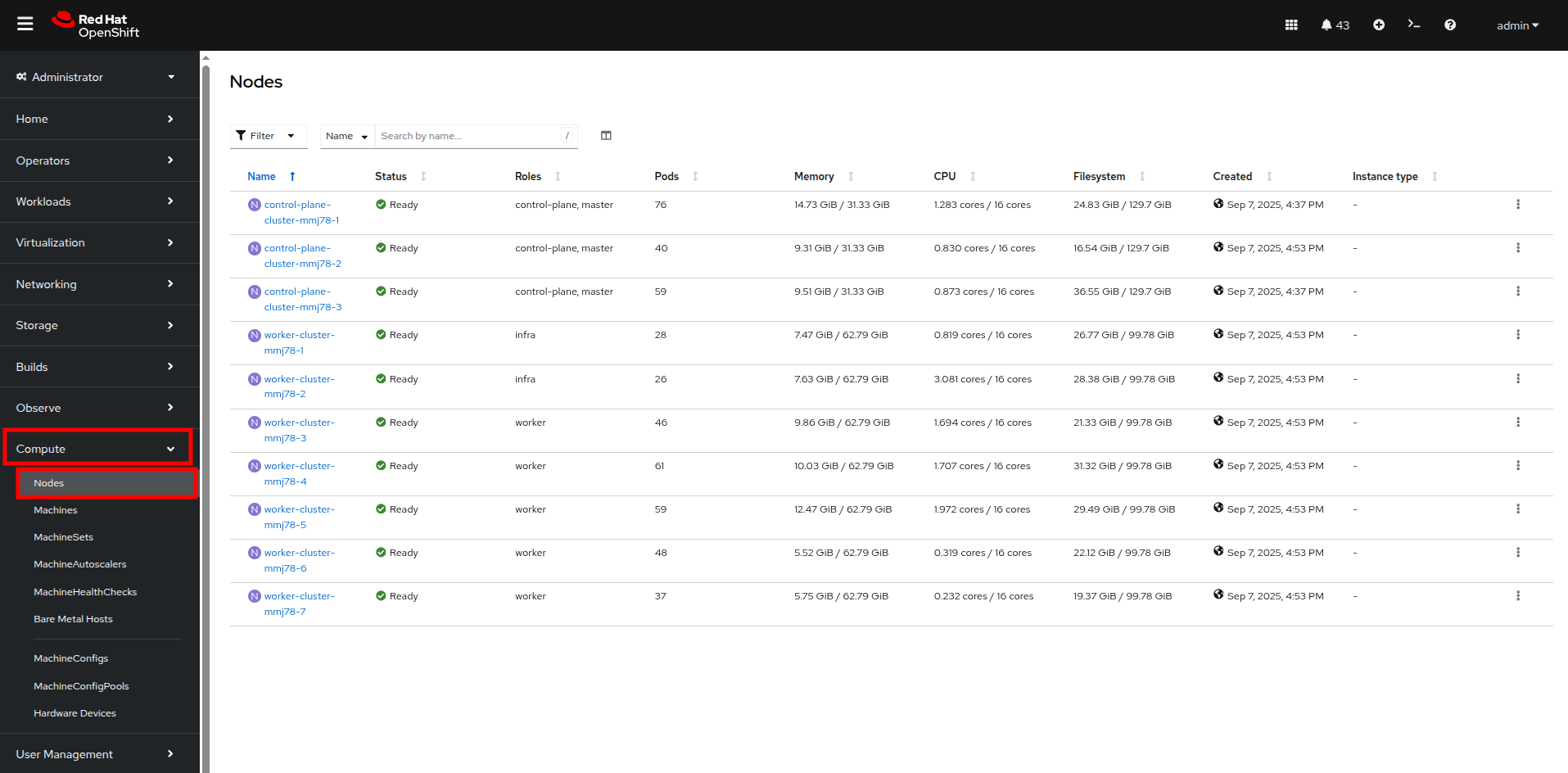 Figure 3. Nodes
 -
Click on your worker node 5 in your cluster. The Node details page comes up where you can see more detailed information about the node.
-
The page shows alerts that are being generated by the node at the top-center of the screen, and provides graphs to help visualize the utilization of the node by displaying CPU, Memory, Storage, and Network Throughput graphs at the bottom-center of the screen.
-
You can change the review period for these graphs to periods of 1, 6, or 24 hours by clicking on the dropdown at the top-right of the utilization panel.
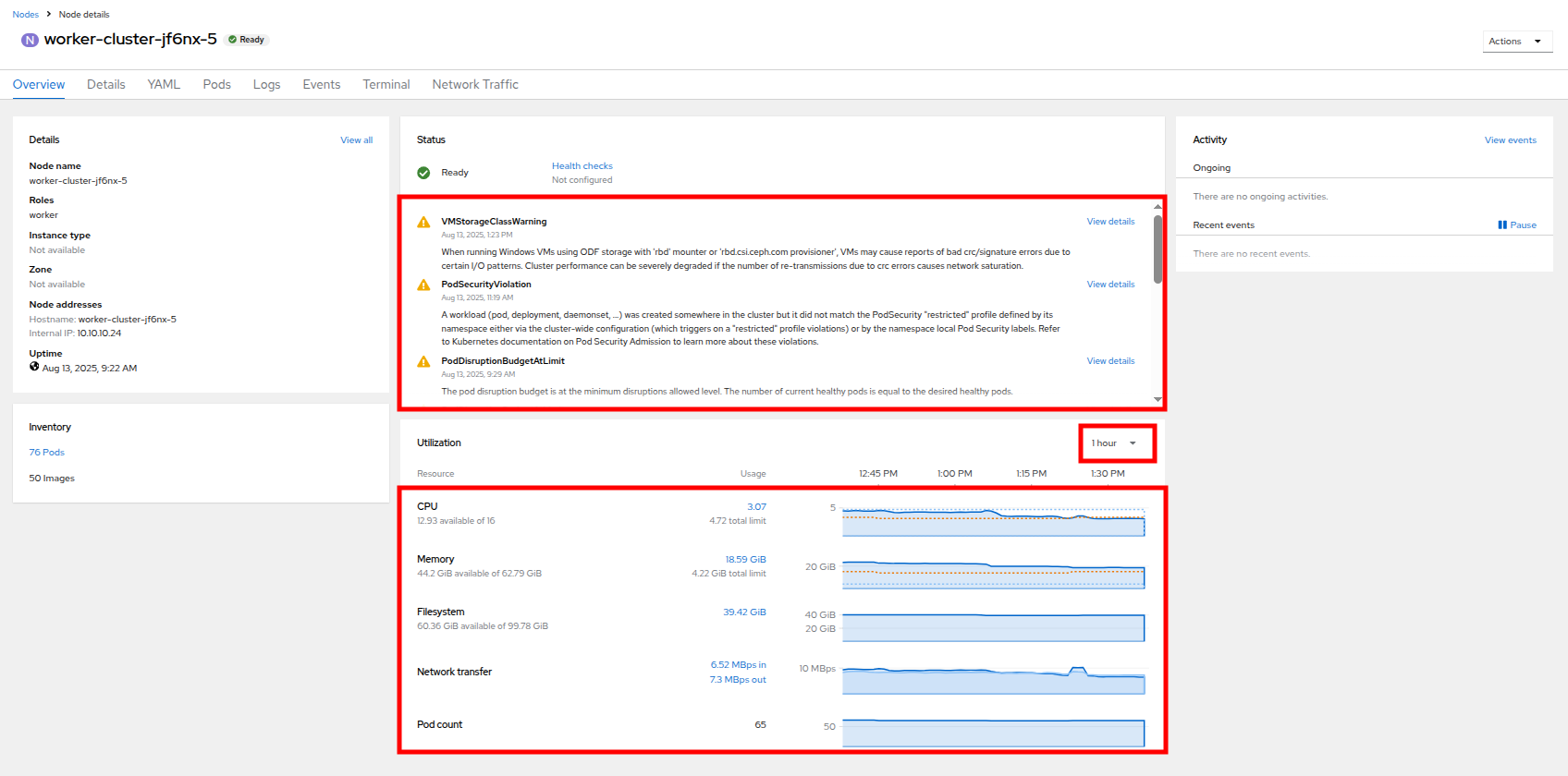 Figure 4. Node Details
 -
You can click on any one of the graphs to see a more detailed version and what queries are being run to display that information. Try now by clicking on the graph for the CPU metrics.
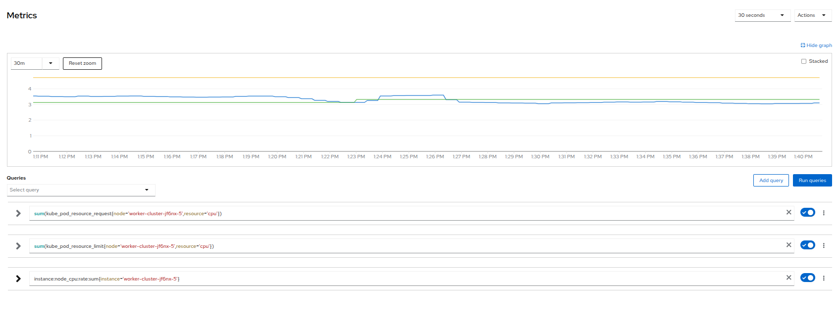 Figure 5. Node Metrics
Virtual Machine Graphs
Outside of the physical cluster resources, it is also very important to be able to visualize what is going on with our applications and workloads like virtual machines. Lets examine the information we can find out about these.
| For this part of the lab, we are going to use an application to generate additional load on some of our virtual machines so that we can see how graphs are generated. |
-
Using the left side navigation menu click on Workloads followed by Deployments.
-
Make sure that you are in the Project: webapp-vms.
-
You should see one pod deployed here called loadmaker.
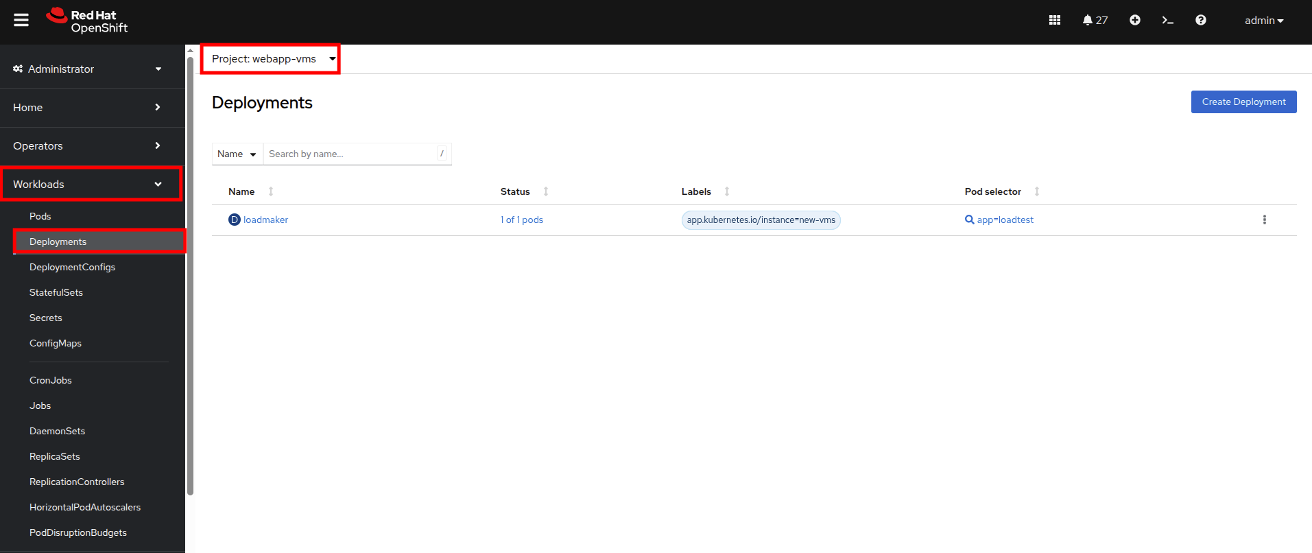 Figure 6. Loadmaker Deployment
 -
Click on loadmaker and it will bring up the Deployment details page.
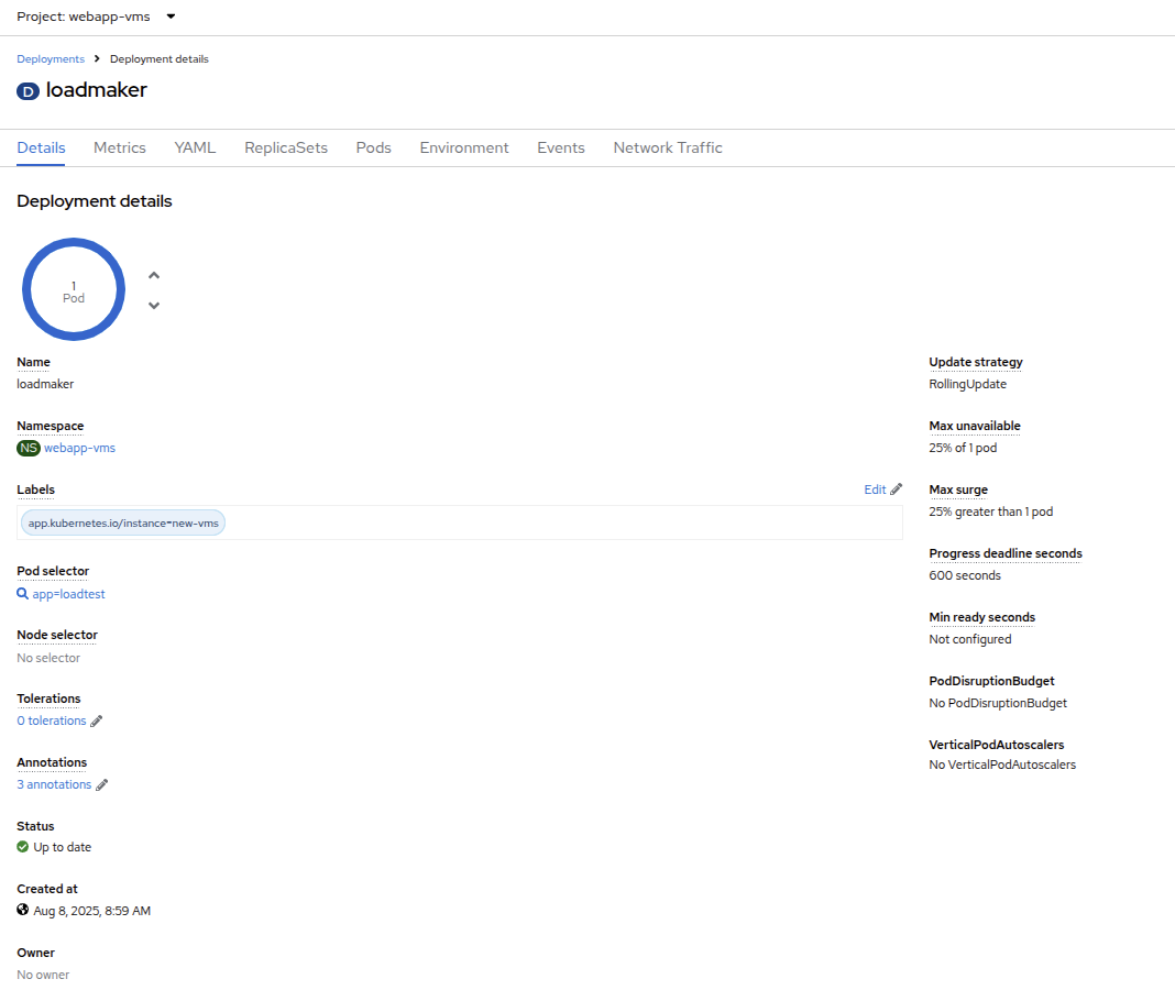 Figure 7. Deployment Details
 -
Click on Environment, you will see a field for REQUESTS_PER_SECOND, change the value in the field to
75and click the Save button at the bottom.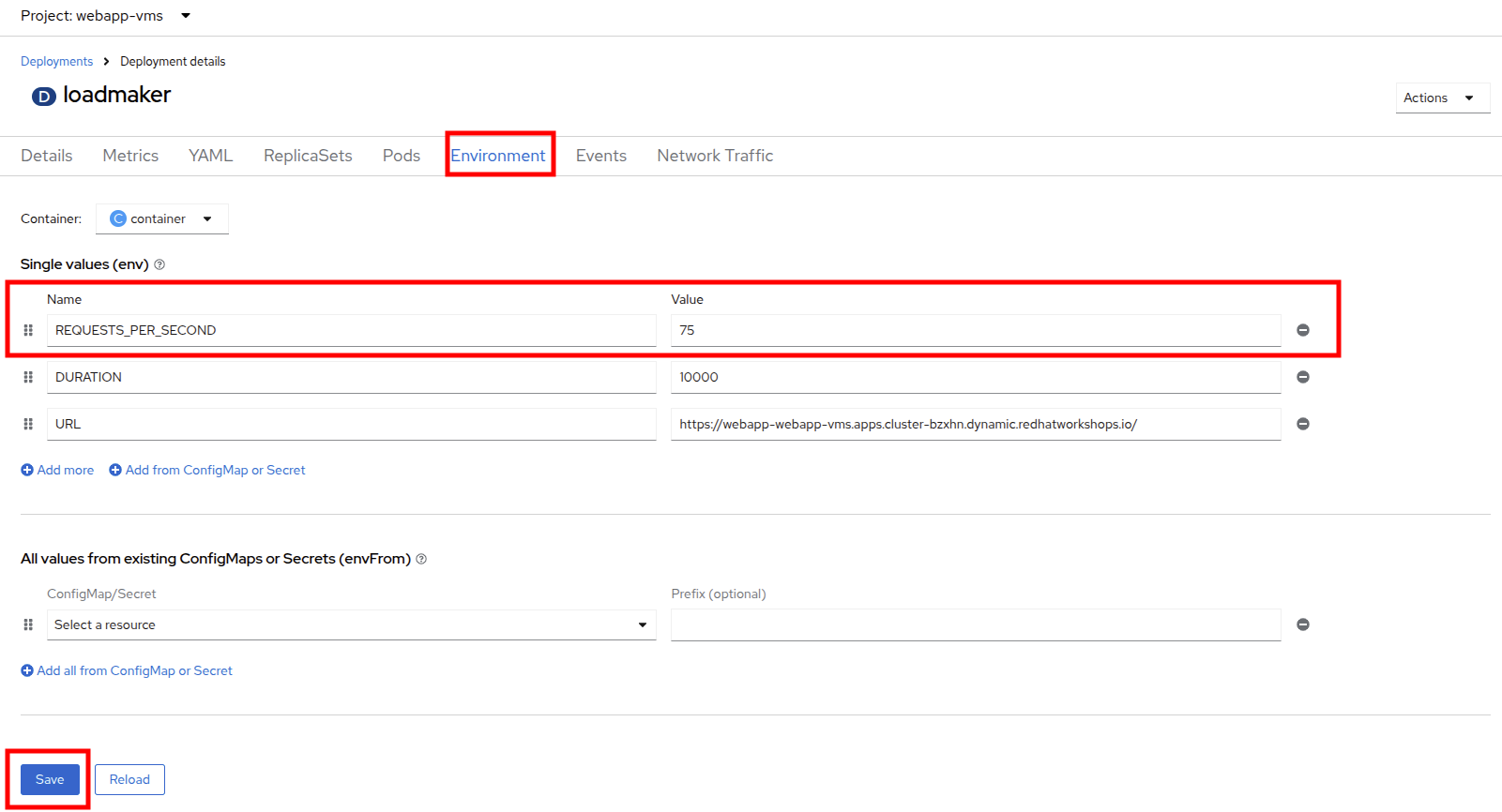 Figure 8. LM Pod Config
 -
Now lets go check on the VMs that we are generating load against.
-
On the left side navigation menu click on Virtualization and then VirtualMachines. Select the webapp-vms project in the center column. You should see three virtual machines: winweb01, winweb02, and database.
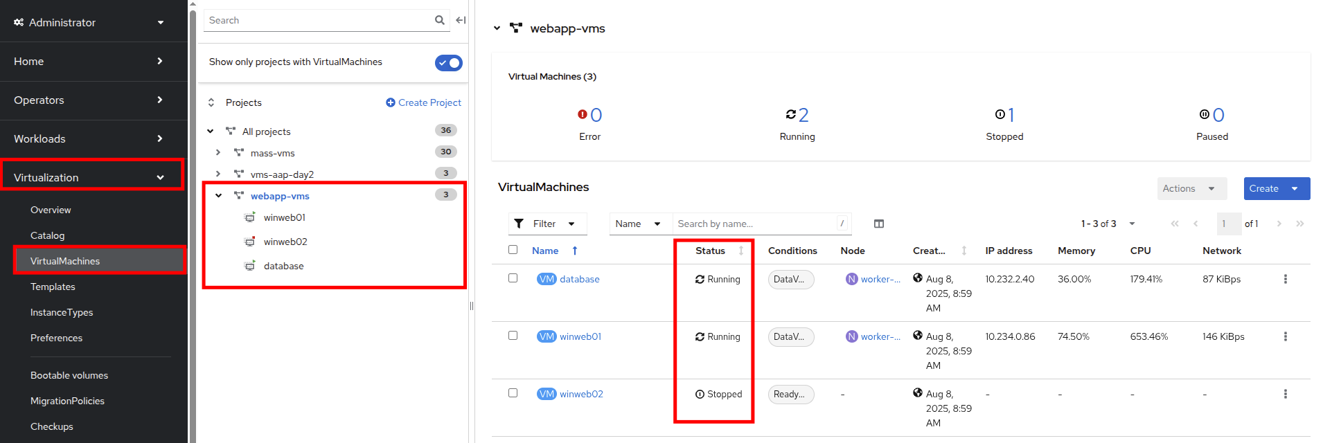 Figure 9. WebApp VMs
At this point in the lab only database and winweb01 should be powered on. If they are off, please power them on now. Do not power on winweb02 for the time being. -
Once the virtual machines are running, click on winweb01. This will bring you to the VirtualMachine details page.
-
On this page there is a a Utilization section that shows the following information:
-
The basic status of the VM resources (cpu, memory, storage, and network transfer) which are updated every 15 seconds.
-
A number of small graphs which detail the VM performance over a recent time period, by default this is the last 5 minutes, but we can select a value up to 1 week from the drop down menu.
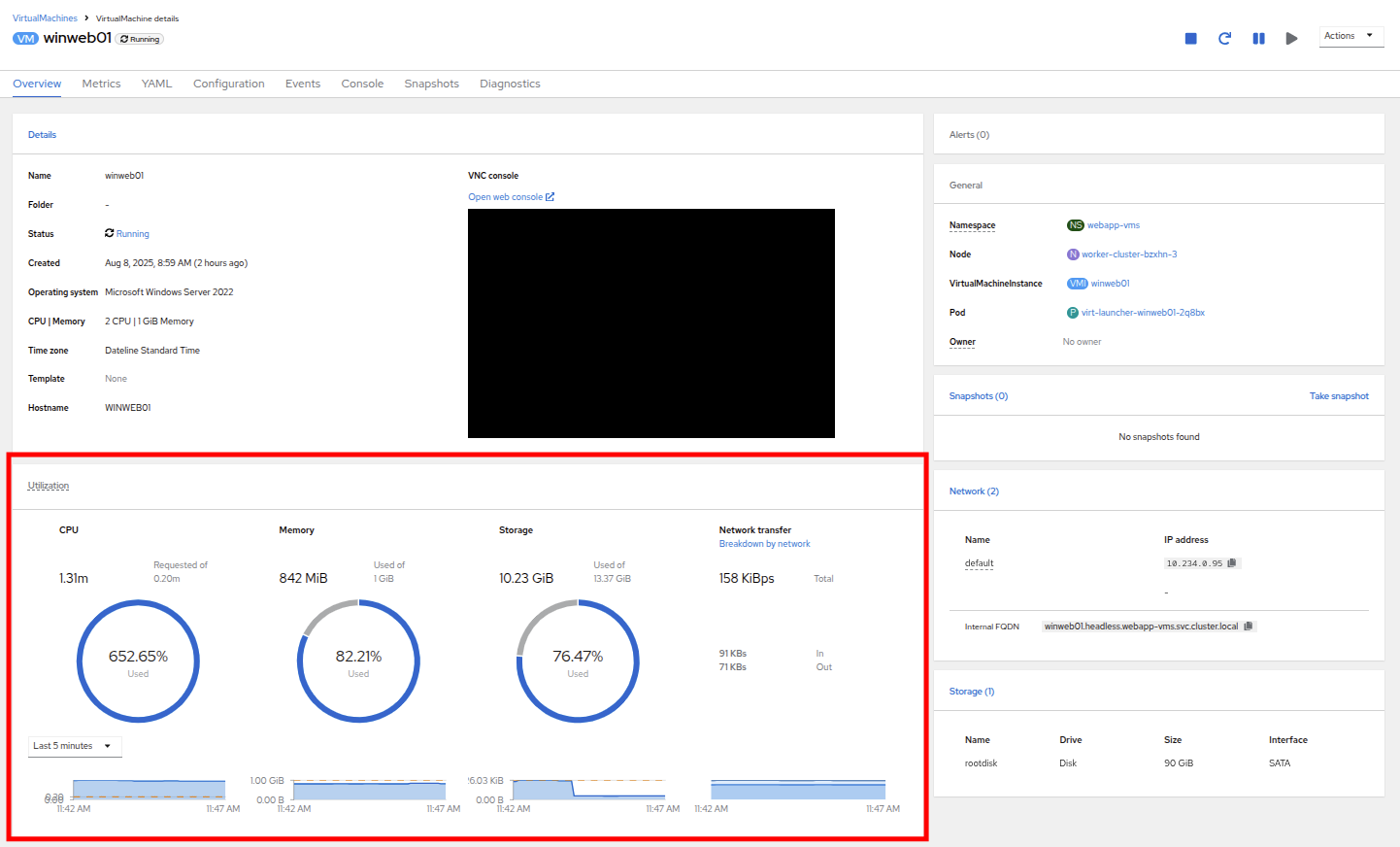 Figure 10. VM Details
-
-
Taking a closer look at Network Transfer by clicking on Breakdown by network you can see how much network traffic is passing through each network adapter assigned to the virtual machine. In this case, the one default network adapter.
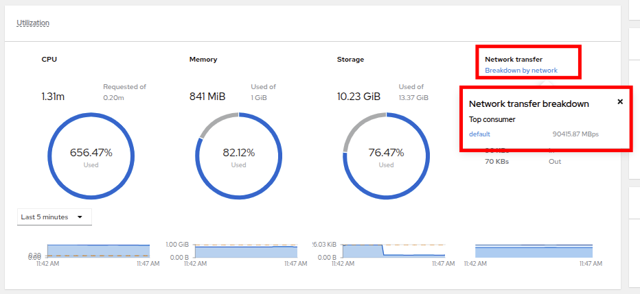 Figure 11. Select Network
 -
When you are done looking at the network adapter, click on the graph showing CPU utilization.
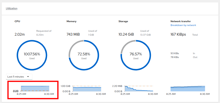 Figure 12. Select CPU
 -
This will launch the Metrics window which will allow you to see more details about the CPU utilization. By default this is set to 30 minutes, which should show the spike in CPU utilization since we’ve turned on the load generator, but you can also click on the drop down and change that to 1 hour in case you need a more distant view.
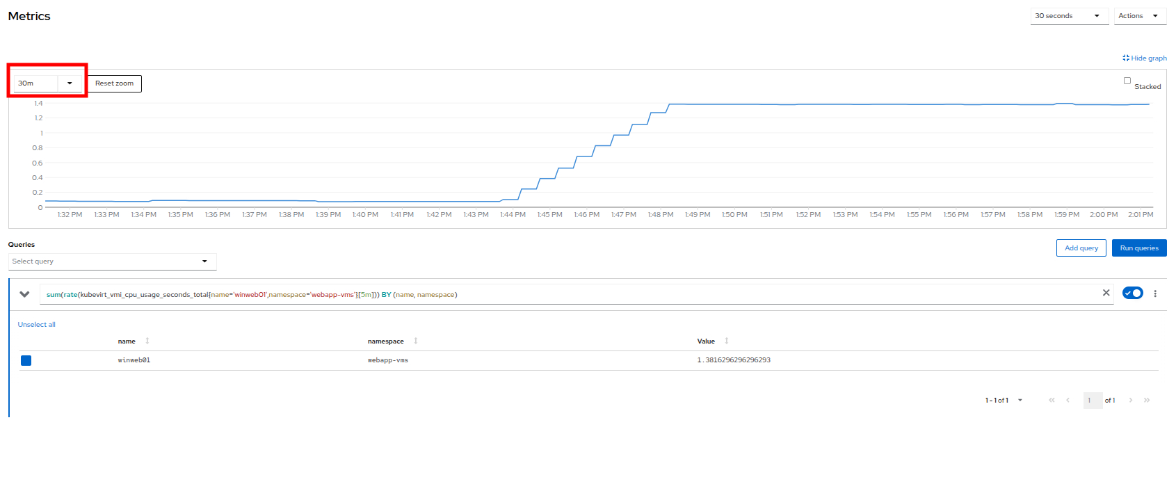 Figure 13. CPU Metrics
 -
You can also modify the refresh timing in the upper right corner.
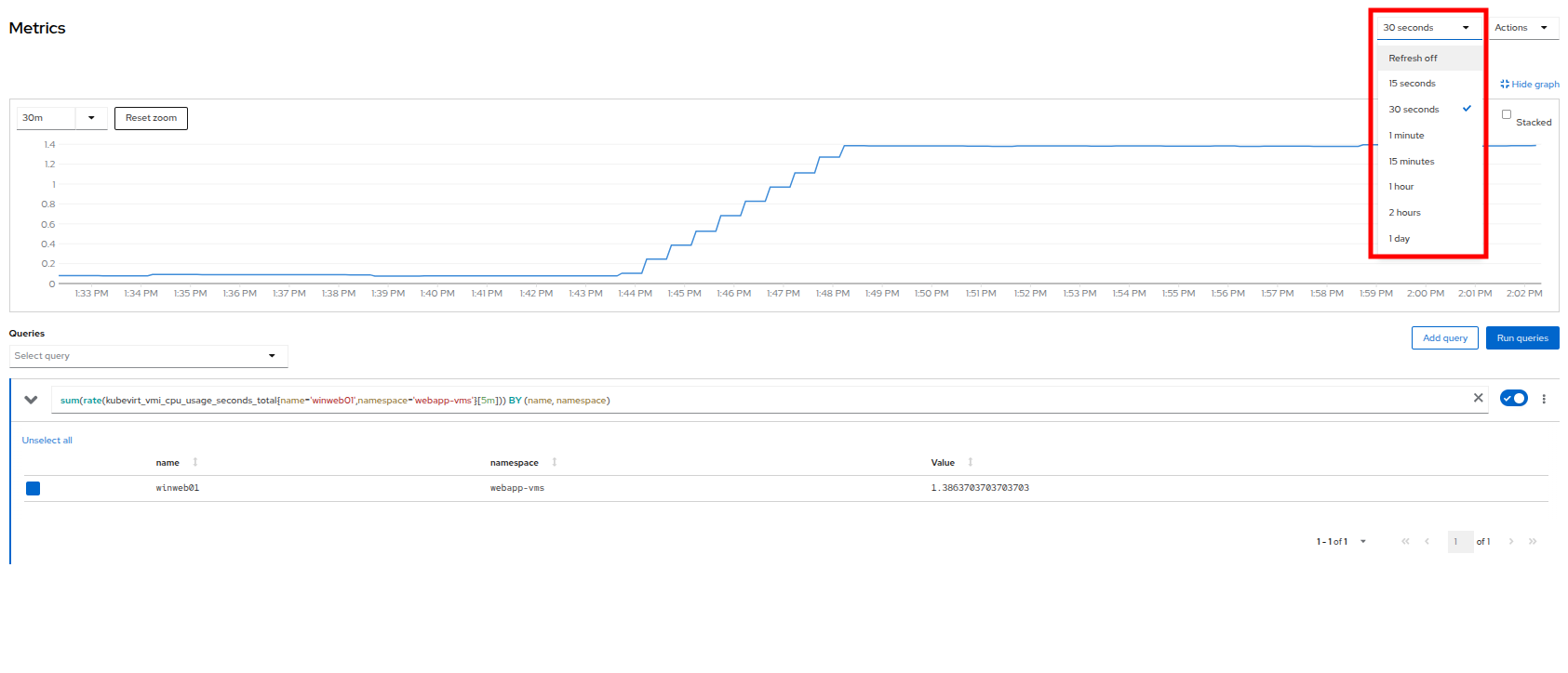 Figure 14. Change Refresh Interval
 -
You can also see the query that is being run against the VM in order to generate this graph, and create your own using the Add Query button.
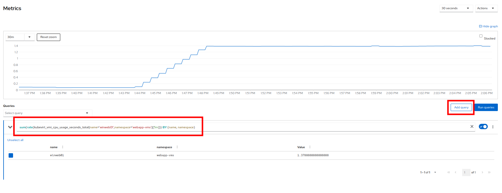 Figure 15. Add_Query
 -
As an exercise, lets add a custom query that will show the amount of vCPU time spent in IO/wait status.
-
Click the Add Query button, and on the new line that appears, paste the following query:
sum(rate(kubevirt_vmi_vcpu_wait_seconds_total{name='winweb01',namespace='webapp-vms'}[5m])) BY (name, namespace) -
Click the Run queries button and see how the graph updates. A new line graph will appear along the bottom of the chart which shows that since the machine has started, there has never been a case where it was not under severe load. Our load generator is working as intended to really hammer the VM.
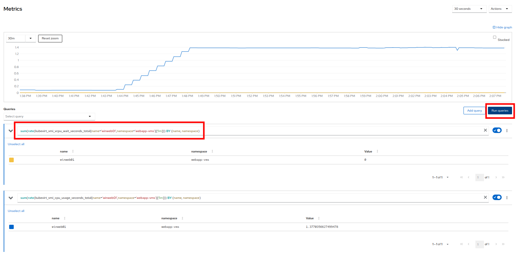 Figure 16. Sample Custom Query
Examining Dashboards
Another powerful feature of OpenShift is being able to use the Cluster Observability Operator to display detailed dashboards of cluster performance. Let’s check some of those out now.
-
From the left side navigation menu, click on Observe, and then Dashboards.
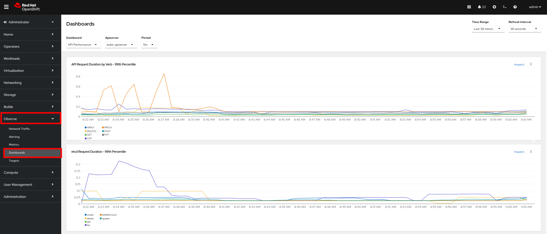 Figure 17. Dashboards
 -
Click on API Performance and search for KubeVirt/Infrastructure Resources/Top Consumers
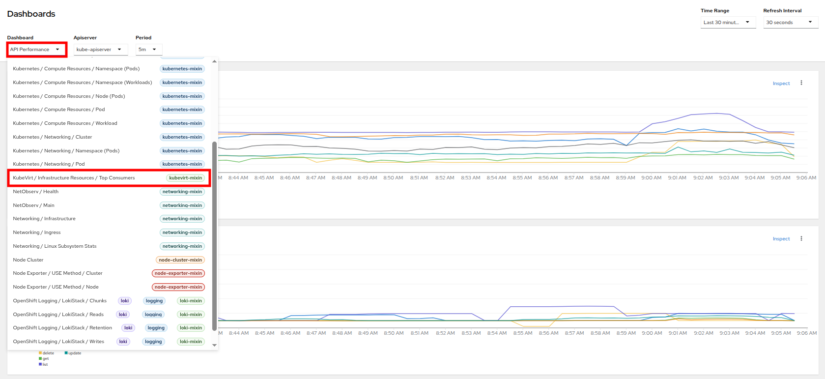 Figure 18. KubeVirt Dashboard
 -
This dashboard will display the top consumers for all of the virtual machines running on your cluster. Look at the Top Consumers of CPU by virt-launcher Pods panel and click the Inspect link in the upper right corner.
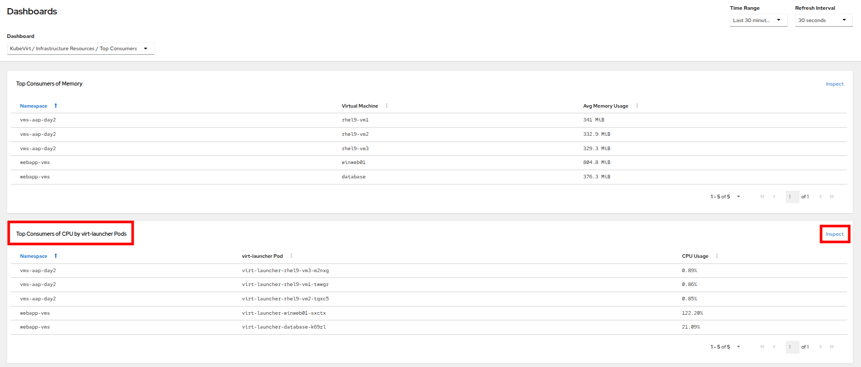 Figure 19. CPU Inspect
 -
You can can select the VMs you want to see in the graph by checking the boxes next to each VM displayed. Notice that winweb01 should show a steady climb in cpu utilization.
-
Try it now by turning some of the lines off. The associated colored line will disappear from the graph when disabled.
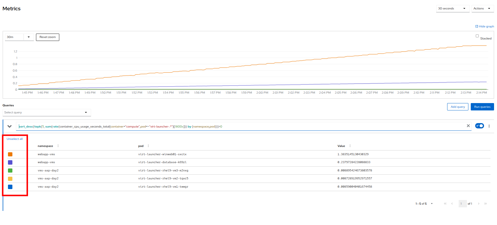 Figure 20. Select Metrics
Now that we have completed this section determining how to locate and display alerts, performance metrics, and graphs about our nodes and workloads, we can leverage these skills in the future in order to troubleshoot our own OpenShift Virtualization environments.
Troubleshooting Resource Utilization on Virtual Machines
The winweb01, winweb02, and database servers work together to provide a simple web-based application that load-balances web requests between the two web servers to reduce load and increase performance. At this time, only one webserver is up, and as we have previously explored is now under high demand. In this lab section we will see horizontally scaling the webservers can help reduce load on the VMs, and how to diagnose this using the metrics, and graphs that are native to OpenShift Virtualization.
-
Click on Virtualization and then VirtualMachines in the left side menu.
-
Now click on winweb01 which should currently be running. This will bring you to the VirtualMachine details page.
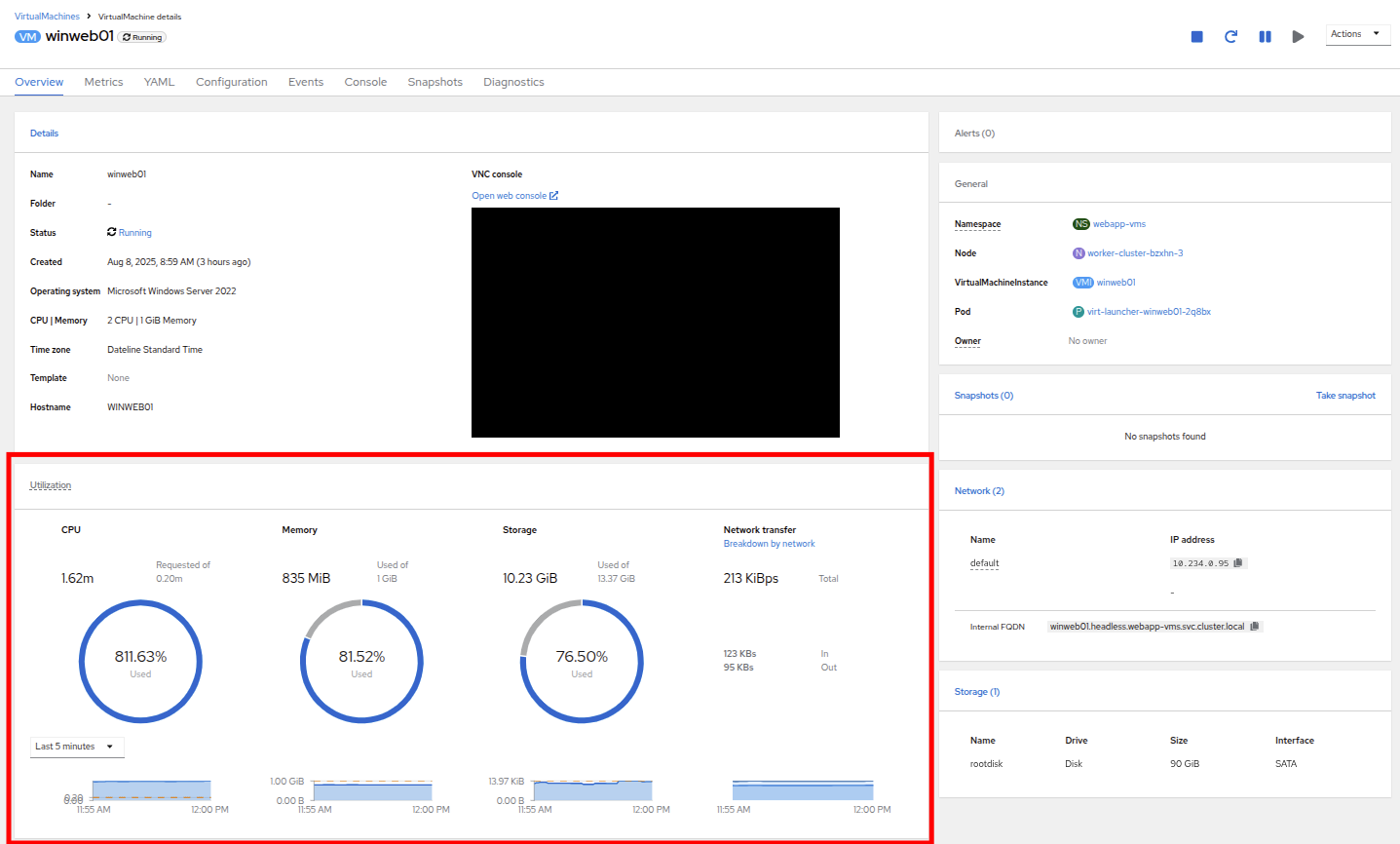 Figure 21. VM Details
 -
Click on the metrics tab and take a quick look at the CPU utilization graph, it should be maxed out.
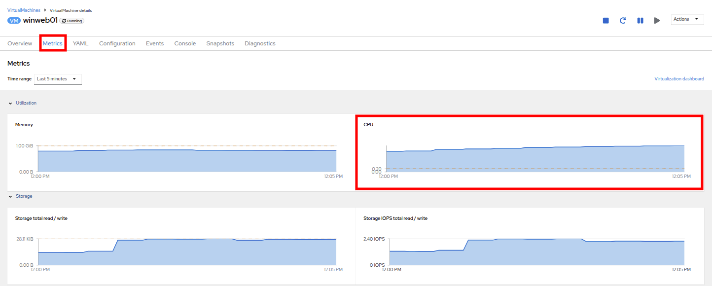 Figure 22. VM Metrics
 -
Click on the CPU graph itself to see an expanded version. You will notice that the load on the server is much higher than 1.0, which indicates 100% CPU utilization, and means that the webserver is severely overloaded at this time.
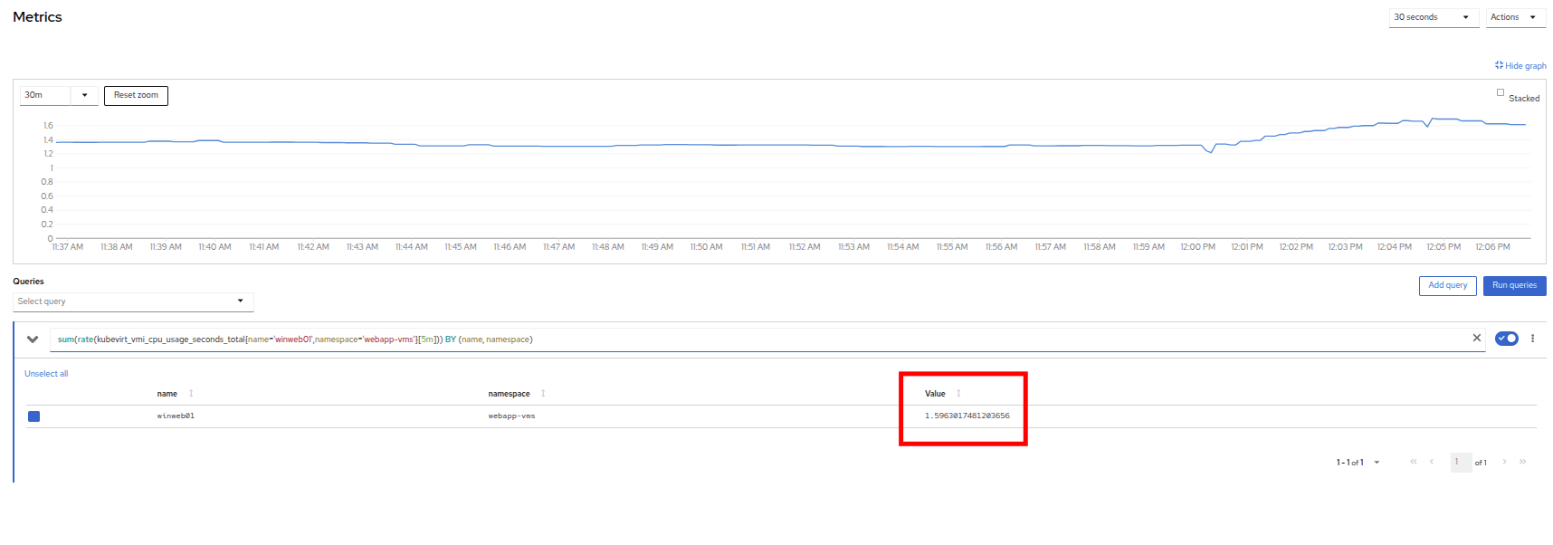 Figure 23. CPU Utilization and Load
Horizontally Scaling VM Resources
-
Return to the list of virtual machines by clicking on VirtualMachines in the left side navigation menu, and click on the winweb02 virtual machine. Notice the VM is still in the Stopped state. Use the Play button in the upper right corner to start the virtual machine.
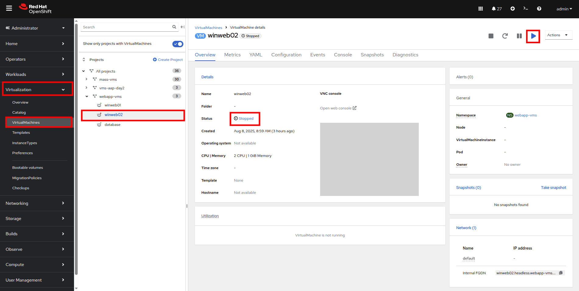 Figure 24. Power On Winweb02
 -
Return to the Metrics tab of the winweb01 virtual machine, and click on its CPU graph again. We should see the load begin to gradually come down.
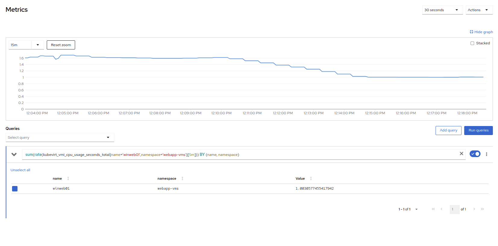 Figure 25. Load Reducing
 -
Add a query to also graph the load on winweb02 at the same time by clicking the Add query button, and pasting the following syntax:
sum(rate(kubevirt_vmi_cpu_usage_seconds_total{name='winweb02',namespace='webapp-vms'}[5m])) BY (name, namespace) -
Click the Run queries button and examine the updated graph that appears.
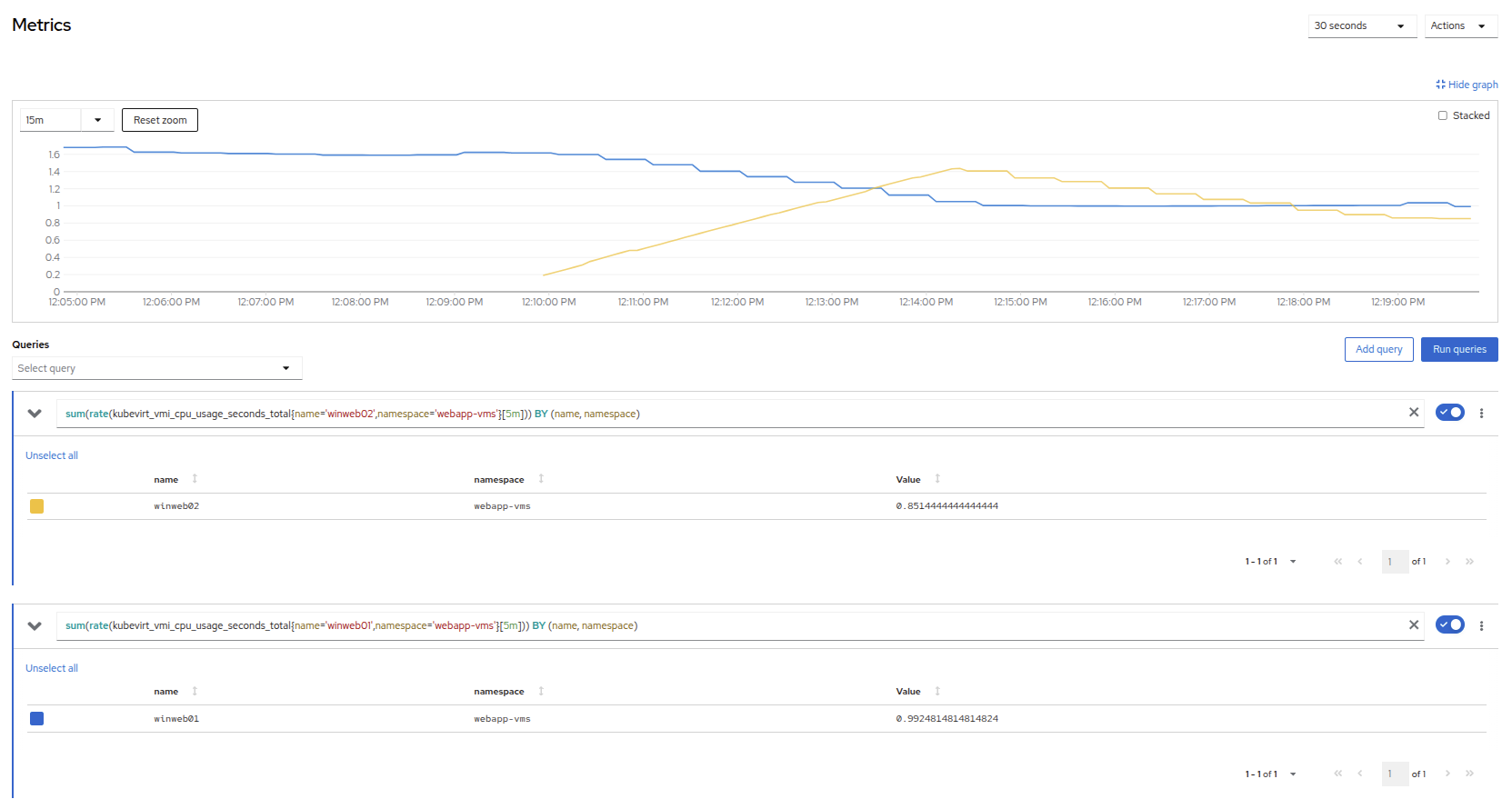 Figure 26. Load Sharing
We can see by examining the graphs that winweb02 is introduced and takes on a large amount of load that winweb01 was originally holding alone. After a few minutes, the load has leveled out between the two virtual machines as they balance the web requests.
Vertically Scaling VM Resources
Even with the load evening out on the VMs over a 5 minute interval, we can still see that they are under fairly high load. Without the ability to scale further horizontally the only option that remains is to scale vertically by adding CPU and Memory resources to the VMs. Luckily as we explored in the previous module, this can be done by hot-plugging these resources, and not affect the workload as it is currently running.
-
Start by examining the graph on the metrics page from the previous section. You can set the refresh interval to the last 5 minutes with the dropdown in the upper left corner. Note that the load on the two virtual guests is holding steady near 1.0, which signifies that both guests are still pretty overwhelmed.
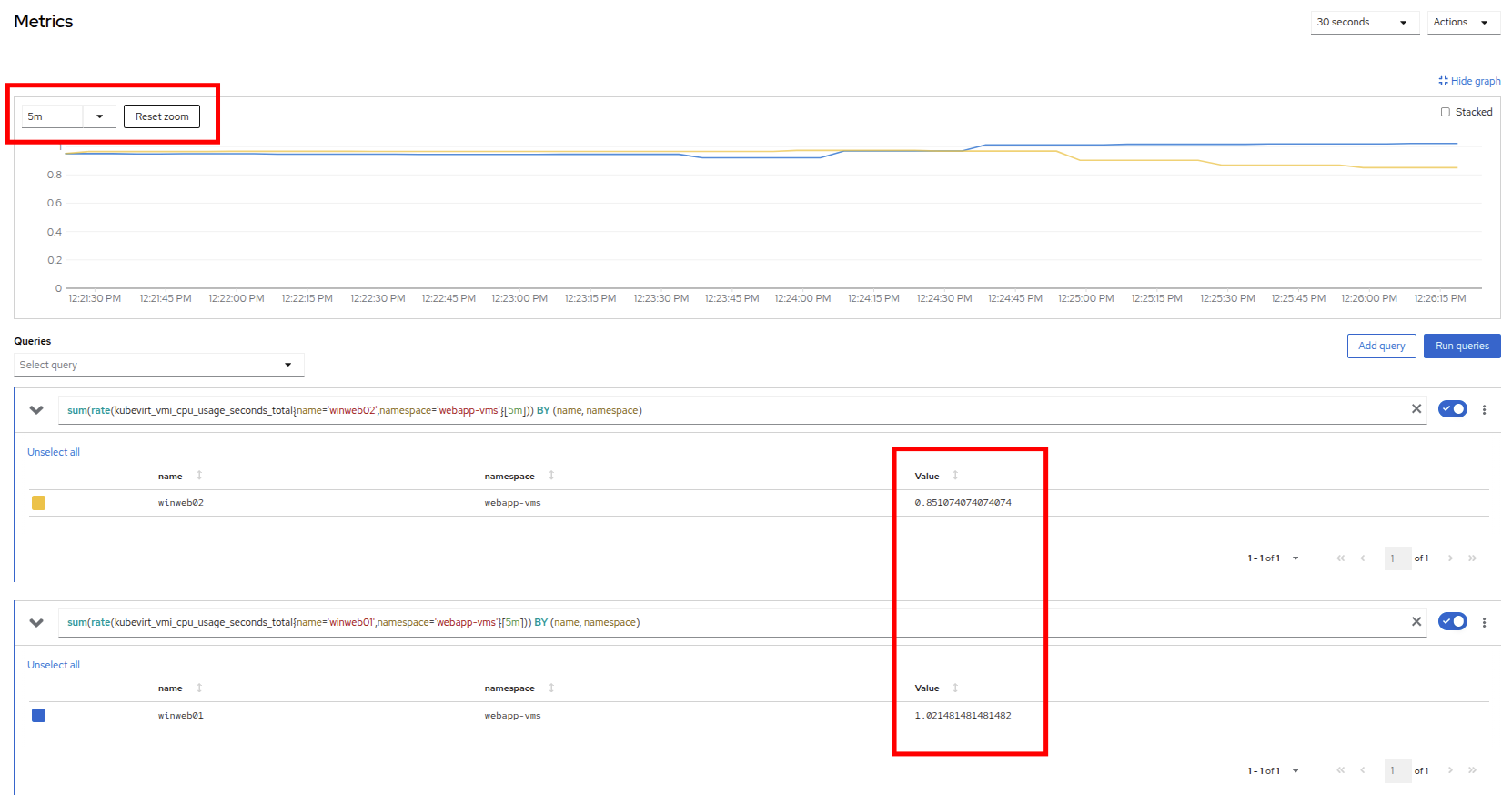 Figure 27. Balanced Load
 -
Navigate back to the virtual machine list by clicking on VirtualMachines on the left side navigation menu, and click on winweb01.
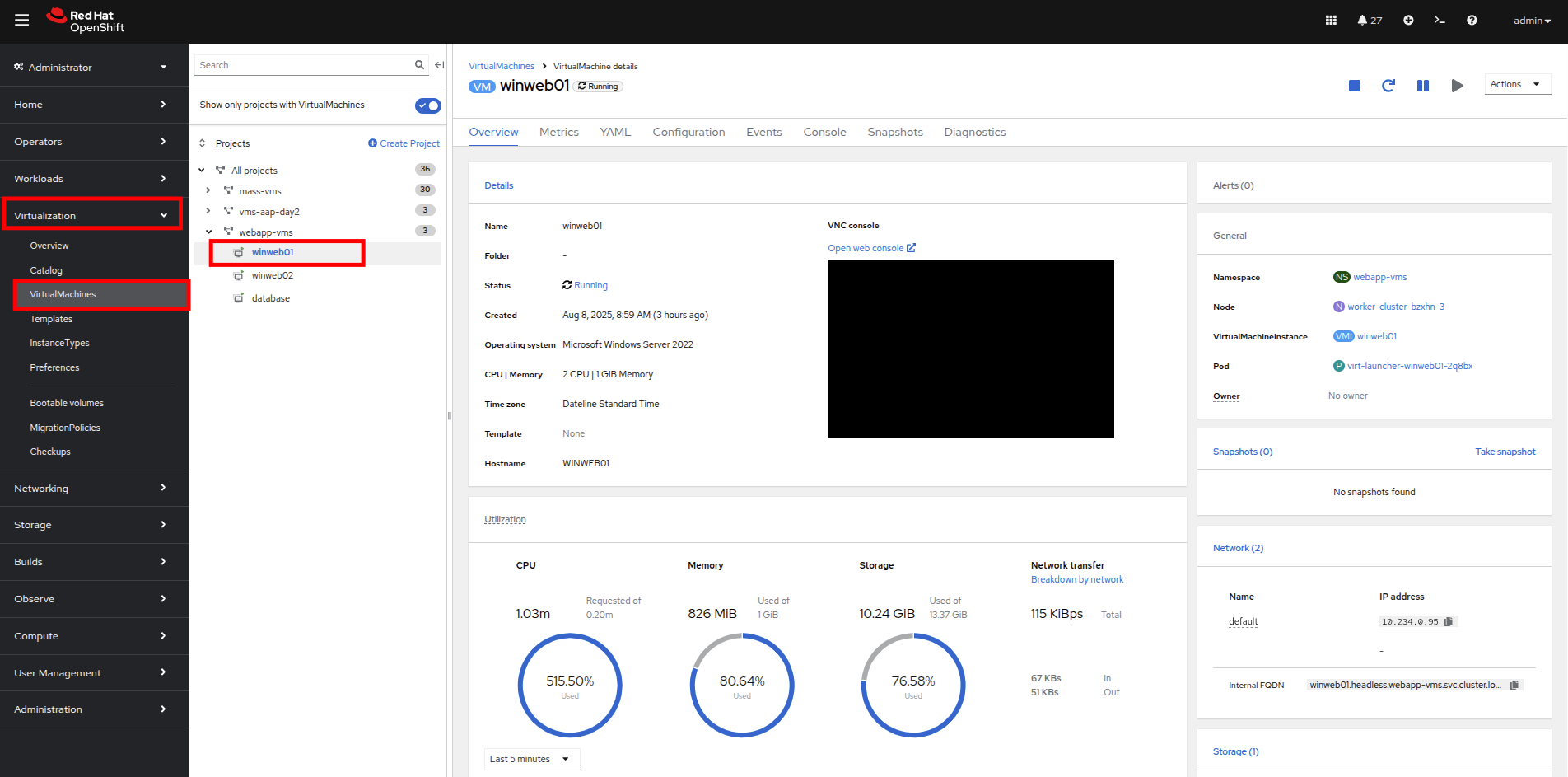 Figure 28. Select VM
 -
Click on the Configuration tab for the VM, and under VirtualMachine details find the section for CPU|Memory and click the pencil icon to edit.
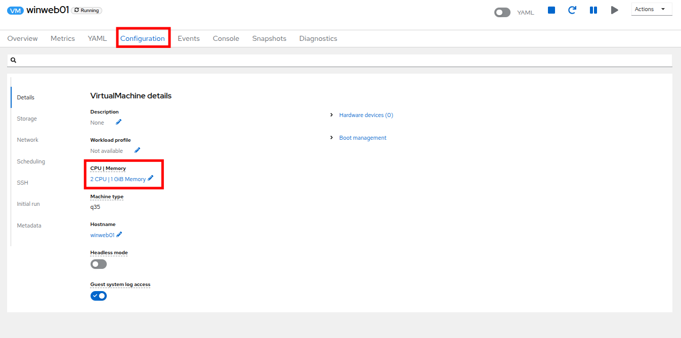 Figure 29. Edit VM
 -
Increase the vCPUs to 4 and click the Save button.
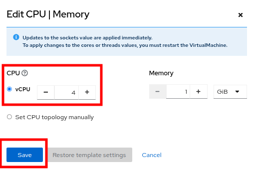 Figure 30. Update Specs
 -
Click back on the Overview tab. You will see that the CPU | Memory section in the details has been updated to the new value, and that the CPU utilization on the guest gradually drops quite quickly now that there are more available resources.
The additional vCPUs you requested might not be available on the OpenShift node the VM is presently deployed on. You might see the VM automatically migrated to another node with adequate vCPU resources.
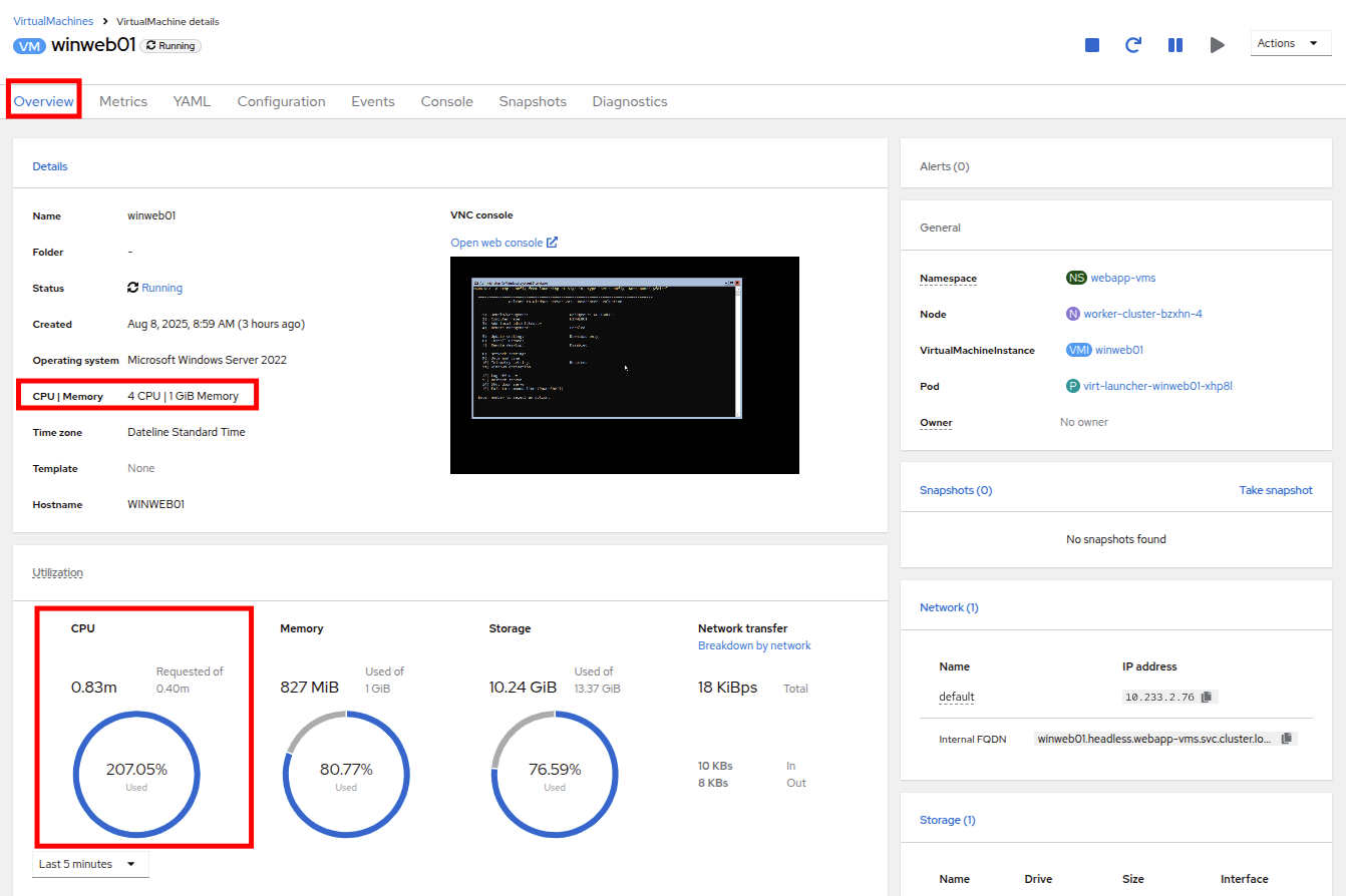 Figure 31. New VM Spec
 -
Repeat these steps for winweb02.
-
Once both vms are upgraded, click on webapp-vms project. You will see that the CPU usage dropped dramatically.
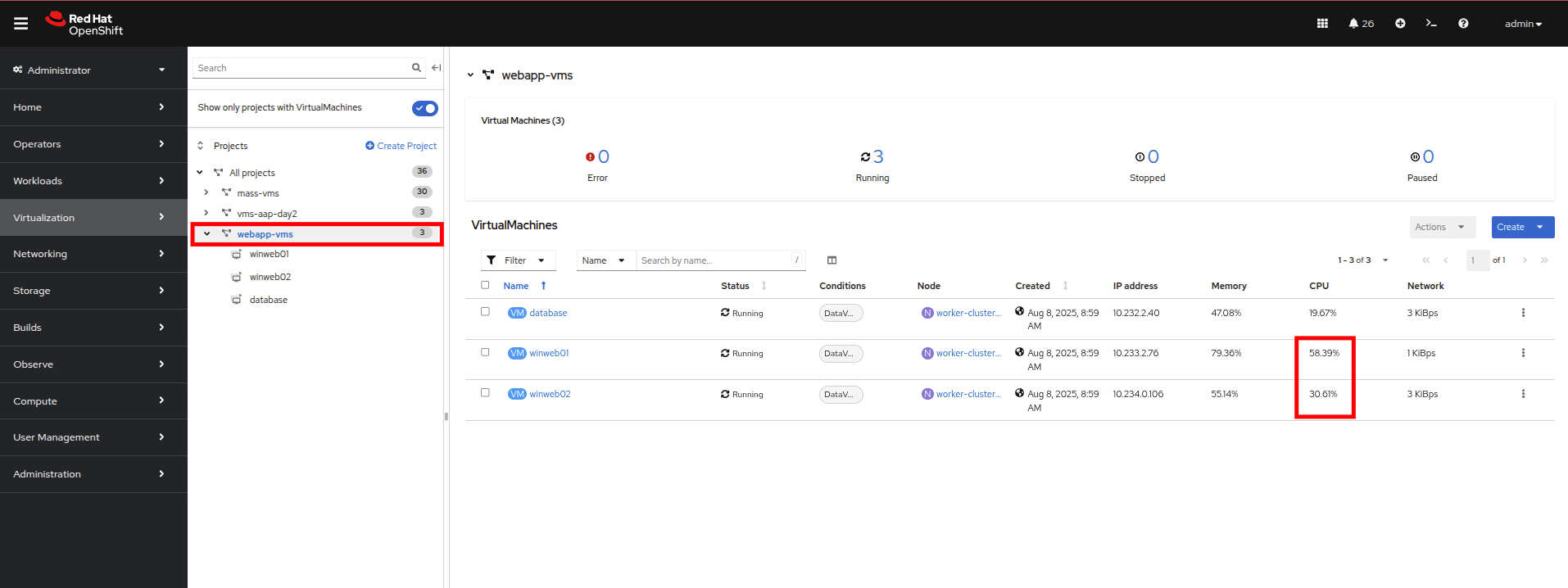 Figure 32. Updated Utilization
 -
Click on winweb01 and then click on the Metrics tab and the CPU graph to view how the utilization graph now looks. You can also re-add the query from winweb02 and see that both graphs came down quite rapidly after the resources on each guest were increased, and the load on each VM is so much less than before.
It might take some time for the actual values to be reflected in the graph. 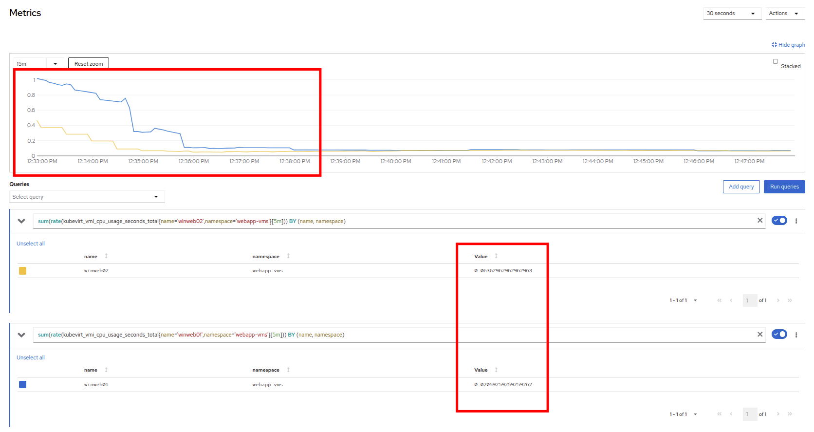 Figure 33. Verify Metrics
Discussing Swap/Memory Overcommit
| This section of the lab is just informative for what we may do in a scenario where we find ourselves out of physical cluster resources. Please read the following information. |
Some times you don’t have the ability to increase CPU or memory resources to a specific workload because you have exhausted all of your physical resources. By default, OpenShift has an overcommit ratio of 10:1 for CPU, however memory in a Kubernetes environment is often a finite resource.
When a normal kubernetes cluster encounters an out of memory scenario due to high workload resource utilization, it begins to kills pods indescriminately. In a container-based application environment, this is usually mitigated by having multiple replicas of an application behind a load balancer service. The application stays available served by other replicas, and the killed pod is reassigned to a node with free resources usually resulting in no noticable effect on the application’s performance to the end user.
This doesn’t work that well for virtual machine workloads which in most cases are not composed of many replicas, and often need to be persistently available.
If you have exhausted the physical resources in your cluster the traditional option is to scale the cluster, but many times this is much easier said than done. If you don’t have a spare physical node on standby to scale, and have to order new hardware, you can often be delayed by procurement procedures or supply chain disruptions.
One workaround for this is to temporarily enable SWAP/Memory Overcommit on your nodes so that you can buy time until the new hardware arrives, this allows for the worker nodes to SWAP and use hard disk space to write application memory. While writing to hard disk is much much slower than writing to system memory, and this is not an ideal scenario, it is possible to enable it for emergency situations, and it does allow you to preserve workloads until additional resources can arrive and be made available.
Scaling a Cluster By Adding a Node.
In an OpenShift cluster, the primary recourse when you have run out of physical resources is to scale the cluster by adding additional worker nodes. This can then allow for workloads that are failing or cannot be assigned to be assigned successfully. This section of the lab is dedicated to just this idea, we will overload our cluster, and then add a new node to allow all of our VMs to run successfully.
| In this lab environment we are not actually adding an additional physical node, we are simulating the behavior by having a node on standby which is tainted to not allow VM workloads. At the appropriate time we will remove this taint, thus simulating the addition a new node to our cluster. |
-
In the left side navigation menu, click on Virtualization and then VirtalMachines.
-
Ensure that all VMs in vms-aap-day2 and webapp-vms projects are powered on.
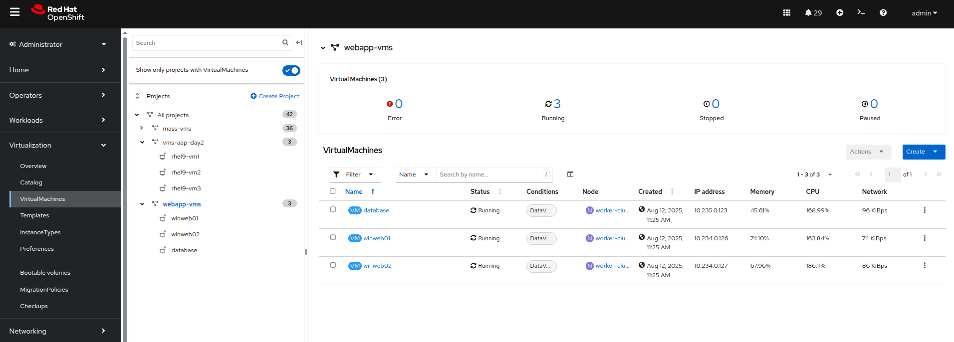 Figure 34. Verify Running VMs
 -
Click on the mass-vm project to list the virtual machines there. Click on 1 - 15 of 36 drop down and change it to 50 per page to display all of the VMs.
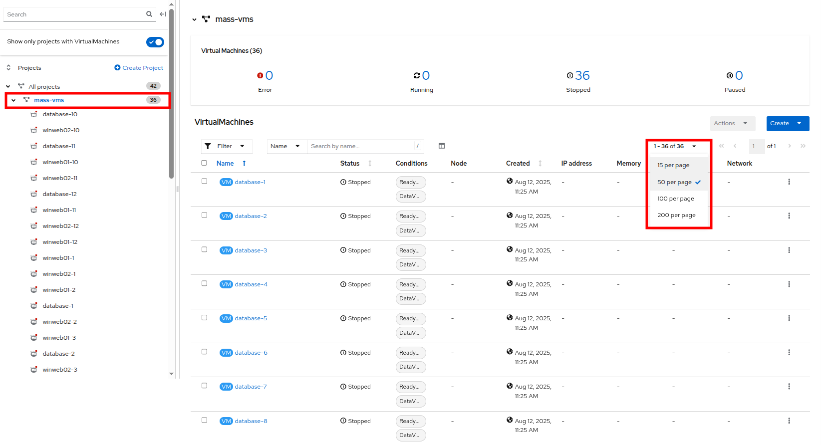 Figure 35. Mass VMs Project
 -
Click on the Check box under the Filter dropdown to select all VMs in the project. Click on the Actions button and select Start from the dropdown menu.
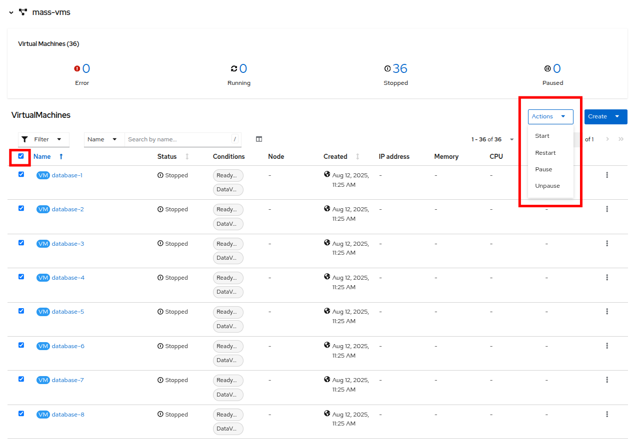 Figure 36. Start All VMs
 -
Once all of the VMs attempt to power on, there should be approximently 5-7 VMs that are currently in an error state.
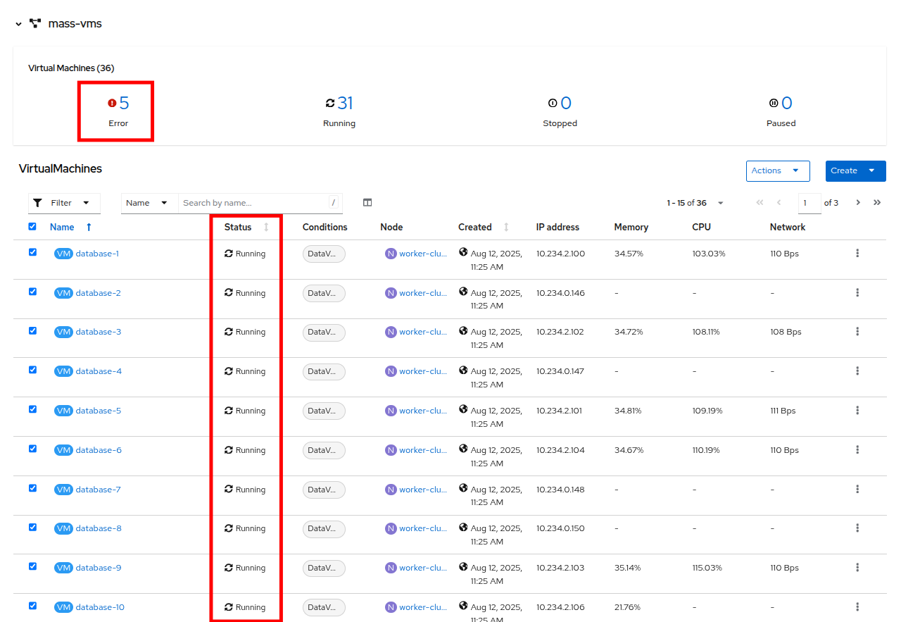 Figure 37. VMs After Startup
 -
Click on the number of errors to see an explanation for the error state.
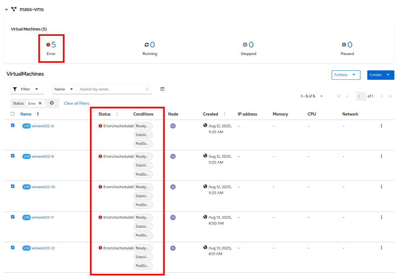 Figure 38. Error Details
 -
Each of these VMs will show a ErrorUnschedulable in the status column, because the cluster is out of resources to schedule them.
-
In the left side navigation menu, click on Compute then click on Nodes. See that three of the worker nodes (nodes 3-5) have a large number of assigned pods, and a large amount of used memory, while worker nodes 6 and 7 are using much less by comparison.
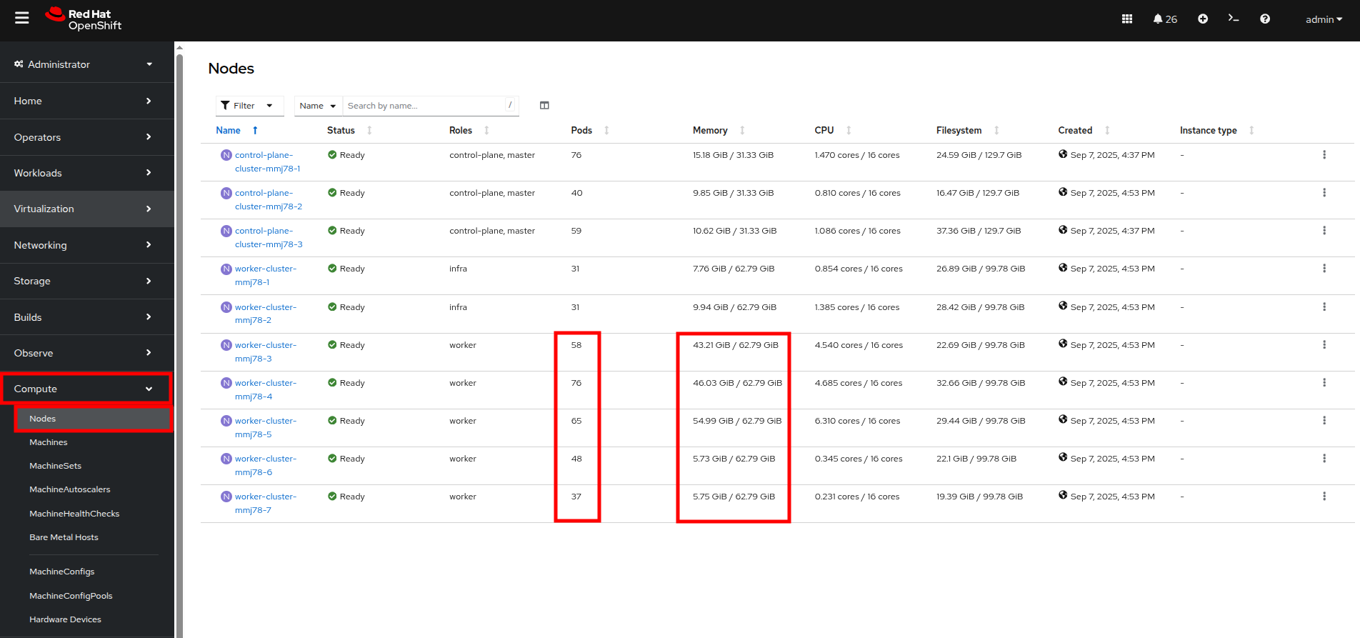 Figure 39. Nodes
In an OpenShift environment, the memory available is calculated based on memory requests submitted by each pod, in this way the memory a pod needs is guaranteed, even if the pod is not using that amount at the time. This is why each of these worker nodes are considered "full" even though they only show about 75% utilization when we look. -
Click on worker node 3, you will be taken to the Node details page. Notice there are warnings about limited resources available on the node. You can also see the graph of memory utilization for the node, which shows the used memory in blue, and the requested amount as an orange dashed line as well.
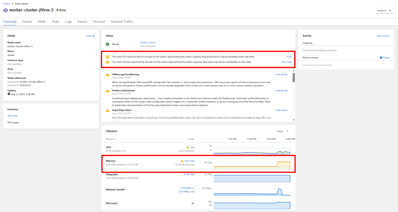 Figure 40. Worker Node 3 Details
 -
Click on the Pods tab at the top, and in the search bar, type
virt-launcherto search for VMs on the node.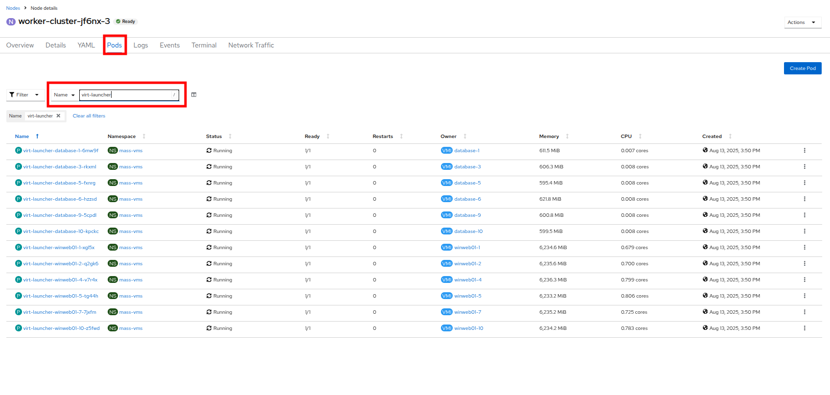 Figure 41. VMs On Worker Node 3
 -
Now, click on Nodes in the left-side navigation menu, and then click on worker node 6 which will bring you to its Node details page. Notice there are no CPU or Memory warnings currently on the node.
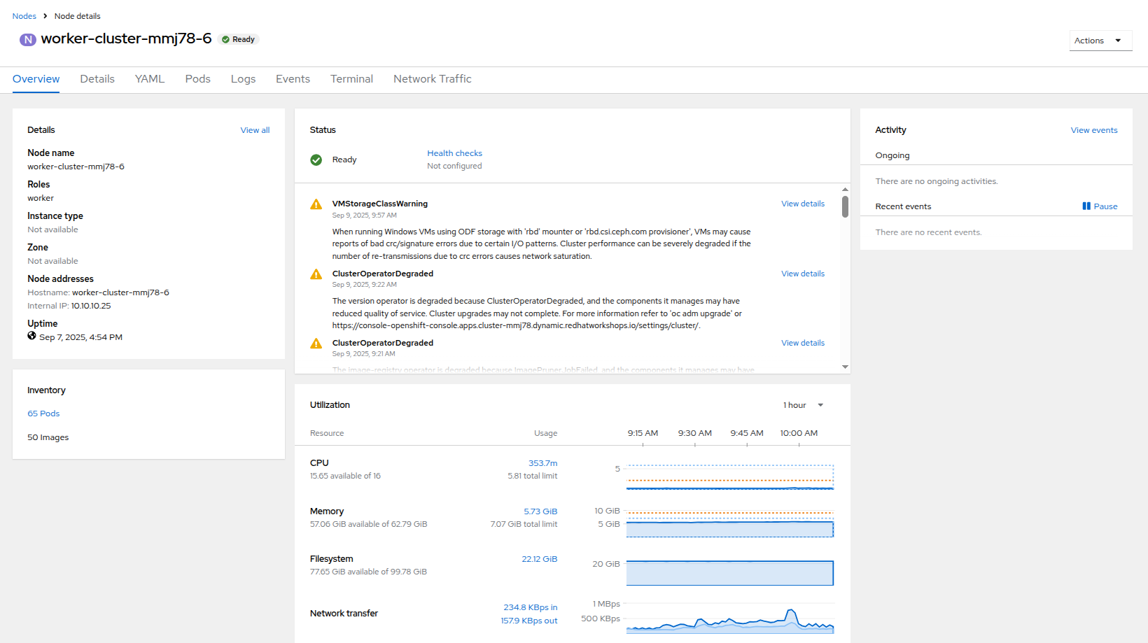 Figure 42. Worker Node 6 Details
 -
Click on the Pods tab at the top, and in the search bar, type
virt-launcherto search VMs on the node. Notice that there are currently none.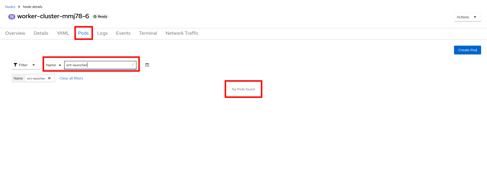 Figure 43. VMs On Worker Node 6
 -
Click on the Details tab, and scroll down until until you see the Taints section where there is one taint defined.
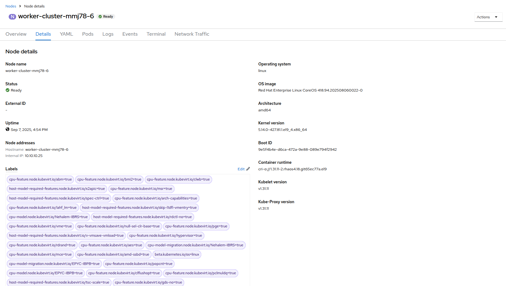 Figure 44. Node Details
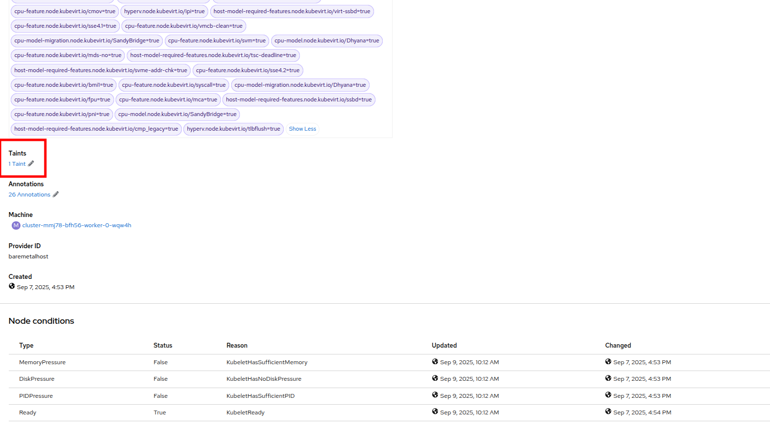 Figure 45. Select Taints
 -
Click on the pencil icon to bring up a box to edit the current Taint on the node. When the box appears, click on the - next to the taint definition to remove it and click the Save button.
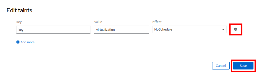 Figure 46. Remove Taint
 -
Once the taint is removed, scroll back to the top and click on the Pods tab again and type
virt-launcherinto the search bar once more, you will see the unscheduleable VMs are being assigned to this node now.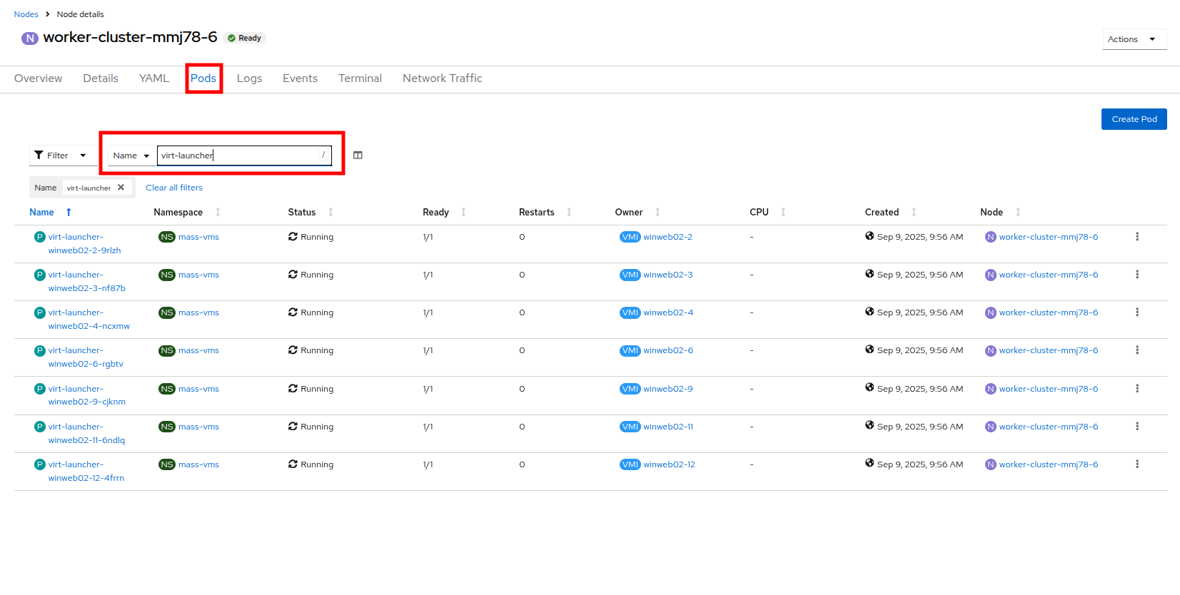 Figure 47. VMs On Worker Node 6
 -
Return to the list of VMs in the mass-vms project by clicking on Virtualization and then clicking on VirtualMachines in the left side navigation menu to see all of the VMs now running.
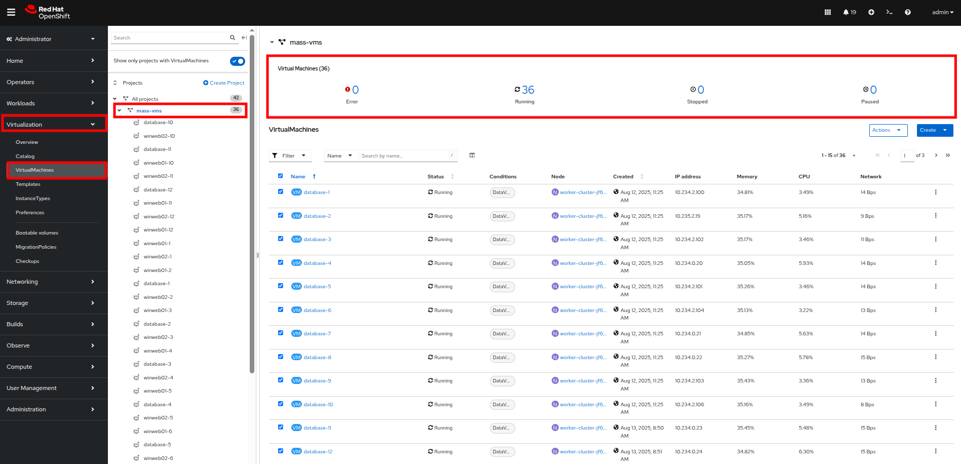 Figure 48. Mass VMs Running
Load Aware Cluster Rebalancing
While we were able to have all of our virtual guests schedule correctly by adding another physical node, we often find that this can leave our node utilization slightly unbalanced across our cluster.
We can check this easily by clicking on the Filter drop down menu and scrolling until we see how the VMs are laid out on each worker node.
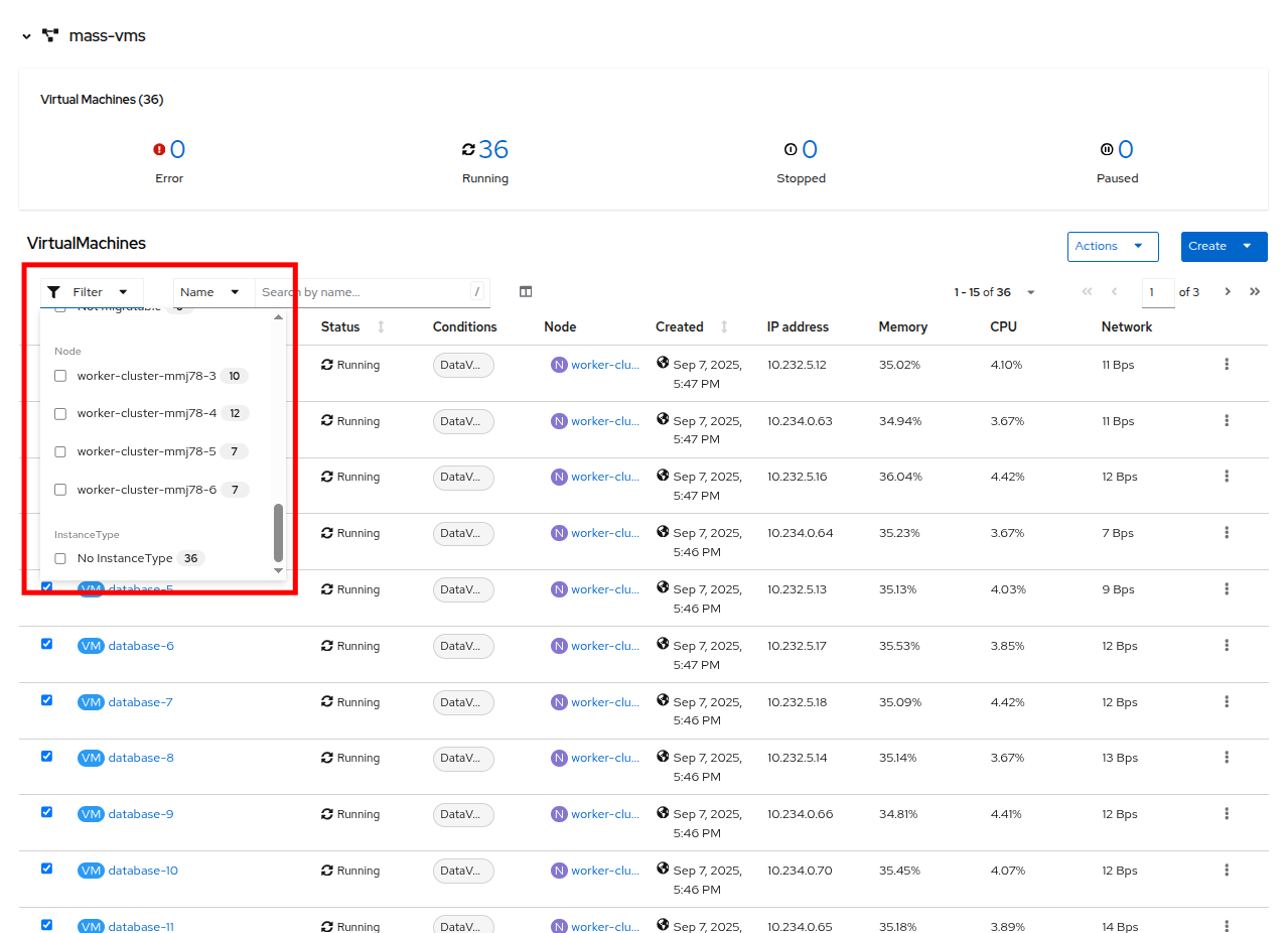
In order to remedy this, another feature we can take advantage of in OpenShift Virtualization is that of making use of the Kube Descheduler operator to rebalance our virtualized workloads across available worker nodes.
In this section we are going to demonstrate OpenShift’s load aware rebalancing feature by introducing another idle node, this time without the cluster being over-provisioned, and we are going to generate load against our virtual machines which will lead to the cluster re-balacing the workloads in an automated fashion.
| Load-aware rebalancing has already been configured on this cluster, this is just an exercise that allows us to see the feature in action. |
Increase Node CPU Utilization
For this section we are going to use the load generator application again, but we have a large number of them deployed in the mass-vms project, we are going to perform some CLI commands to scale the deployments to put pressure on our cluster, and to check the status of rebalancing efforts.
-
To get started, click the icon in the upper right corner to launch the OpenShift Web Terminal. The web terminal will launch at the bottom of your screen.
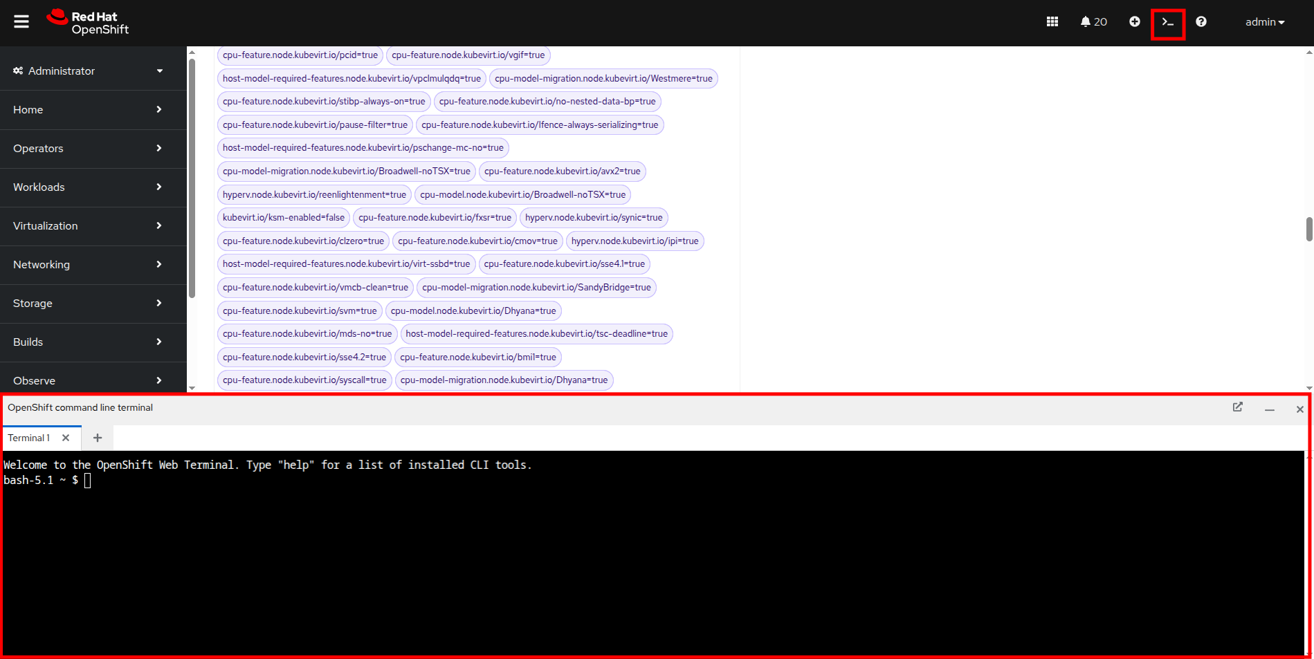 Figure 50. OpenShift Web Terminal
 -
Paste the following syntax into the terminal in order to increase the number of load generator instances to put additional pressure on the cluster.
for i in {1..12}; do oc scale deployment/loadmaker-$i --replicas=6 -n mass-vms; done -
This should start putting additional pressure on each of our virtual machines in the mass-vms project and in turn the nodes hosting them.
-
If we now scale our cluster resources by adding an additional node, the cluster will attempt to balance out our resources by live migrating virtual machines.
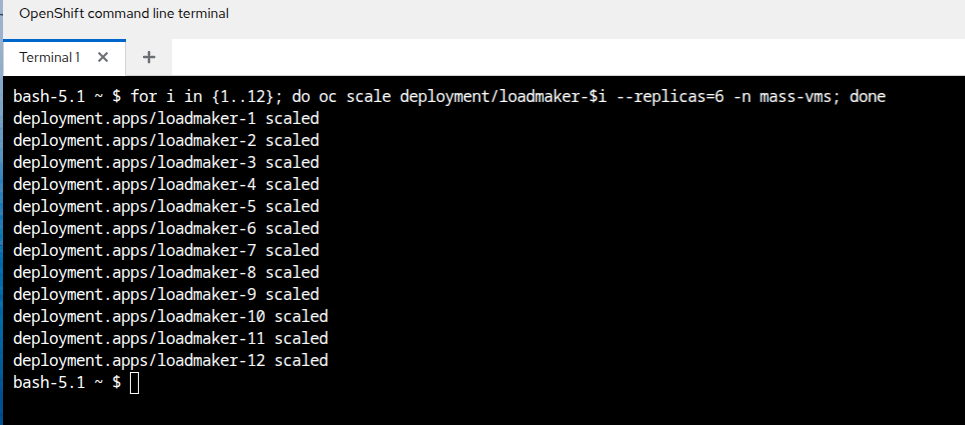 Figure 51. CLI Scale Deployment
Add an Additional Node to the Cluster
-
The first step we want to perform is to repeat the step we did in the earlier section by removing the taint from worker node 7 in our cluster. Do so by clicking on Compute followed by Nodes and click on worker node 7.
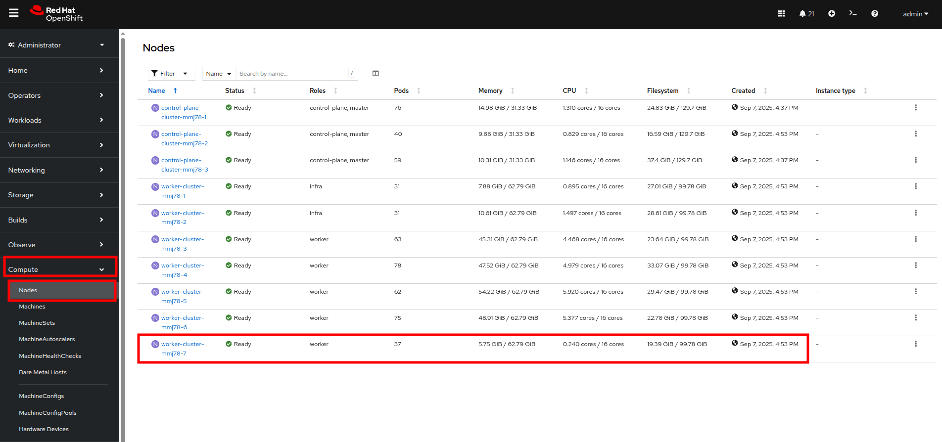 Figure 52. Compute Node List
 -
On worker node 7, to introduce it as a virtual machine host in our cluster, we are going to do as we did previously by clicking on the Details tab.
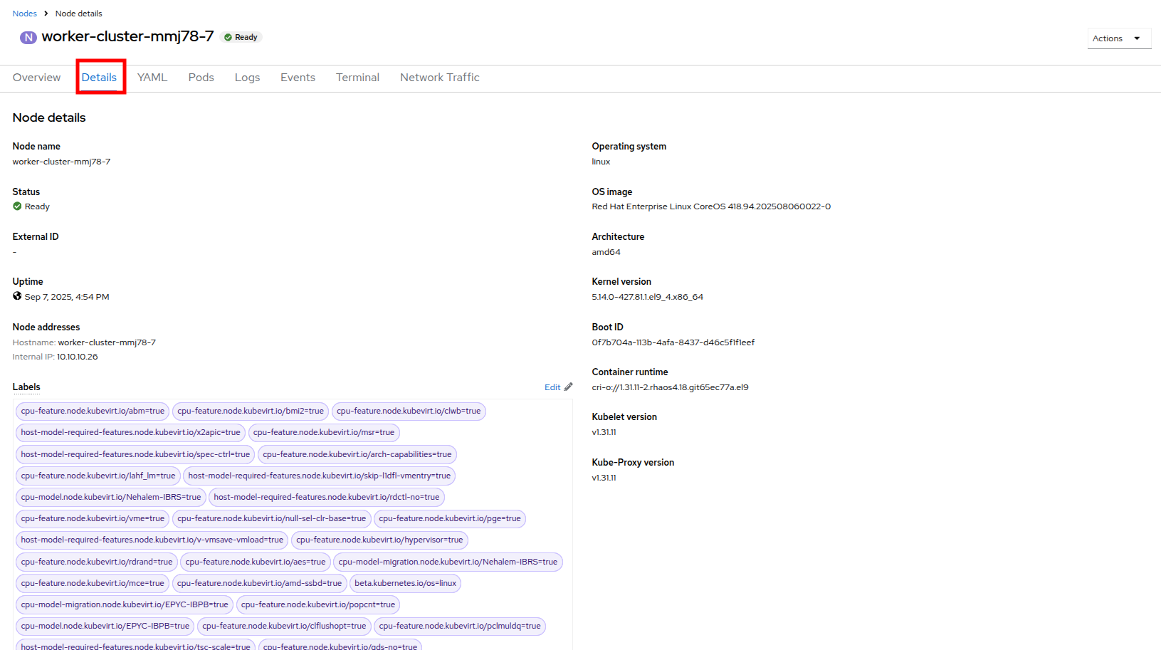 Figure 53. Node 7 Details
 -
Scroll down under the Labels section and you will see the Taints section with one taint listed and a pencil icon next to it. Click the pencil icon to edit the node taint.
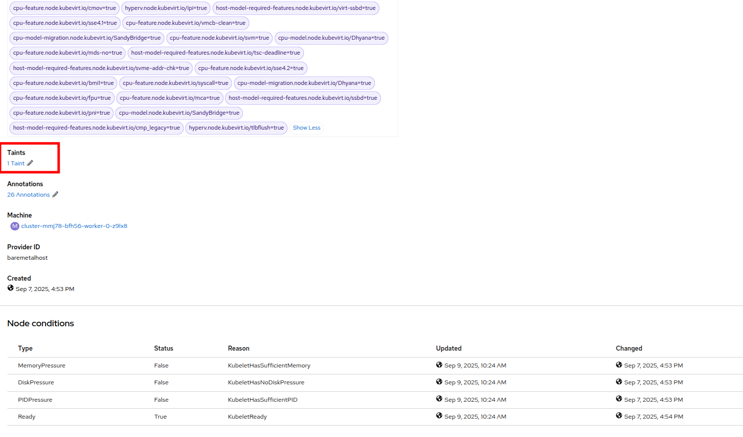 Figure 54. Node 7 Taint
 -
In the window that pops up, click the minus sign to remove the taint, and then click the Save button.
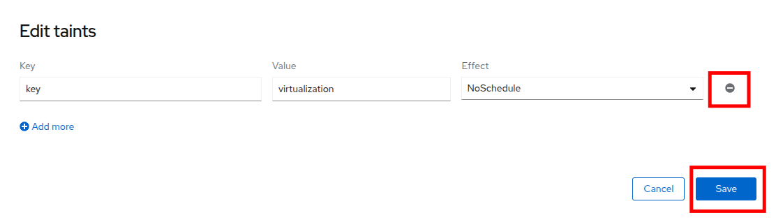 Figure 55. Remove Taint Window
 -
Return to the virtual machine view by clicking on Virtualization and VirtualMachines in the left side menu, click on All projects and finally click on the Filter drop down.
-
You can watch this view update in realtime, in a minute or two node 7 should appear and its guest count should begin to rise as VMs are live migrated to the node to balance out the cluster
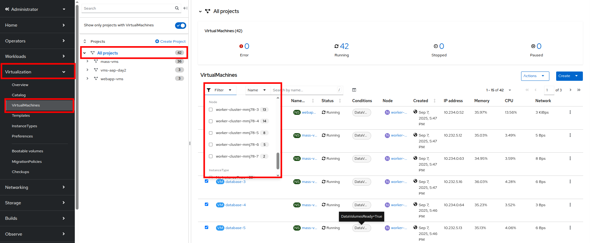 Figure 56. VMs On Node 7
Default configuration for load-aware rebalacing is to refresh every 5 minutes, but for our lab we’ve tuned this variable to 30 seconds to make it easier to visualize in a shorter time period. -
You can also check on the status of any node evacuations across all namespaces by running the following command in the OpenShift Web Terminal.
oc get vmim -AThe command above has a long history and may show quite a view VM evacuations as we have scaled the cluster multiple times during this module. 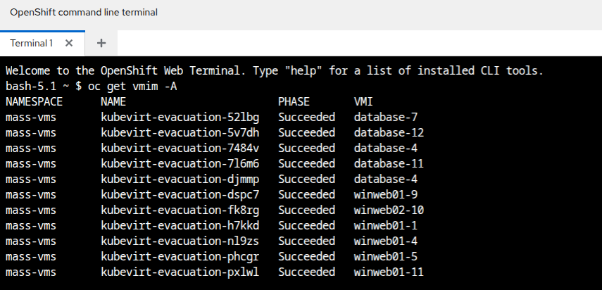 Figure 57. KubeVirt Evacuation List
| In order for the rest of the lab to complete without issues we need to scale back down the load generator pods so that they aren’t causing an adverse effect on the environment. Please do so with the following syntax: |
for i in {1..12}; do oc scale deployment/loadmaker-$i --replicas=0 -n mass-vms; doneSummary
In this module you have worked as an OpenShift Virtualization administrator needing to simulate a high load scenario which you were able to remediate by horizontally and vertically scaling virtual machine resources. You also were able to solve an issue where you had run low on physical cluster resources and were unable to provision new virtual machines by scaling up your cluster to provide additional resources. Lastly you saw that you could further test the boundaries of your physical cluster by generating additional load and observing your virtual machines' ability to perform load-aware balancing across your now expanded cluster.