Module 5: Agent & LLM evaluations (Evals)
|
This module is optional. If you completed Modules 1-4, you have a strong observability foundation. This module adds advanced quality assurance capabilities for those who want deeper expertise in evaluation frameworks or have additional time. |
Observability tells you if your system is working, but evaluations tell you if your agents are working well. Without evals, a 20% drop in answer quality can go unnoticed for weeks until customers complain. In this module, you’ll go beyond basic observability by running LLM evaluations against the Fed Aura Capital prospect agent using MLflow’s evaluation framework, Prompt Registry, and LLM-as-a-Judge scorers (using one LLM to evaluate another LLM’s output quality).
| In this module, you’re wearing your AI Developer / Engineer hat, focusing on model output quality, prompt management, and evaluation design. |
This is the AI Developer’s quality assurance layer, the inner loop where you manually evaluate agent outputs during development. In Module 6, you’ll automate this into an outer loop that detects regressions continuously.
Learning objectives
By the end of this module, you’ll be able to:
-
Launch a Jupyter workbench in Red Hat OpenShift AI
-
Register versioned prompts in MLflow’s Prompt Registry
-
Create evaluation datasets with inputs and expected outputs
-
Run deterministic and LLM-as-a-Judge evaluations against a live agent
-
Analyze evaluation results and per-trace assessments in MLflow
Why evaluations matter for AgentOps
In the Fed Aura Capital mortgage system, agents make consequential decisions:
-
The prospect agent qualifies leads. A false negative loses a $300K mortgage sale.
-
The underwriter agent assesses risk. A $500K bad loan approval creates regulatory exposure.
-
The underwriter agent checks compliance. Violations risk legal penalties and license suspension.
In production, even a 1% error rate means 100 failures per day on 10,000 daily interactions. Metrics tell you the agent responded. Traces tell you how it responded. Evaluations tell you if it responded correctly.
Exercise 1: Launch a Jupyter workbench
To run evaluations, you need a Jupyter environment. Red Hat OpenShift AI provides managed workbenches with pre-installed data science libraries.
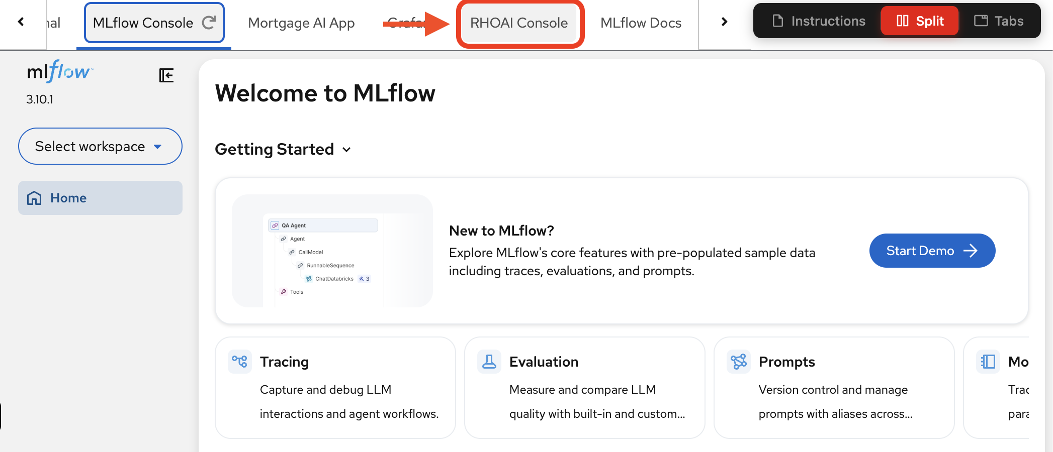
| Throughout this workshop, all key services are accessible as tabs at the top of this page — no need to open separate browser windows. Navigate to the RHOAI Console tab to access the Red Hat OpenShift AI dashboard. |
-
Navigate to the RHOAI Console tab:
-
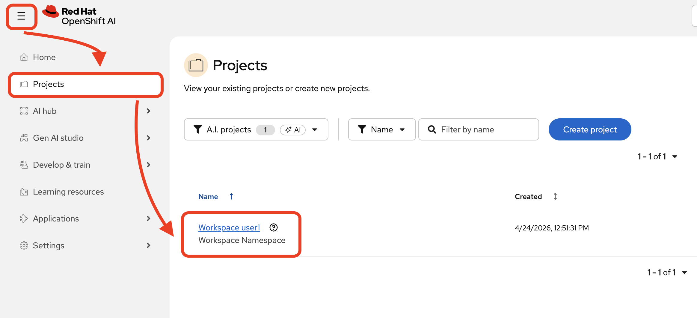
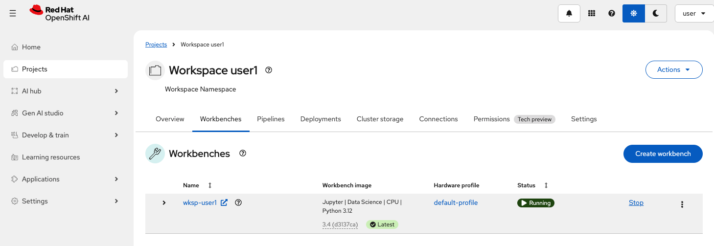
In the Red Hat OpenShift AI (RHOAI) dashboard, navigate to Projects and select your workspace (
wksp-user1).
-
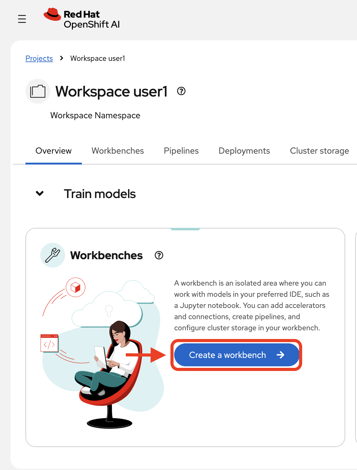
Click Create a workbench:
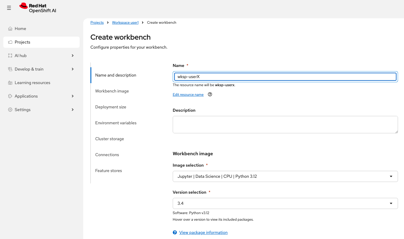
Now, configure it:
-
Name:
wksp-user1 -
Image selection:
Jupyter | Data Science | CPU | Python 3.12 -
Version selection:
3.4 -
Leave other settings as defaults
-
-
Click Create workbench and wait for it to start.
The workbench image download can take a couple of minutes the first time. Please be patient while it pulls the container image and starts. -
Once the status shows Running, click to launch JupyterLab:
| JupyterLab opens in a new window. Use your browser’s split tab feature to view both JupyterLab and these instructions side-by-side, or toggle between windows as you work. |
Exercise 2: Clone the repository and open the evaluation notebook
This is the inner loop in action: as an AI Developer or Engineer, you use Jupyter notebooks to experiment with prompts, tweak agent behavior, and evaluate outputs interactively. The notebook gives you a fast feedback cycle: change a prompt, re-run the evaluation, inspect the results, and iterate, all before any code reaches a pipeline or production.
| Want to learn more about MLflow’s evaluation framework? Open the MLflow Docs tab at the top of this page and explore the Evaluation & Monitoring section, which covers scorers, datasets, and evaluation-driven development workflows in depth. |
The evaluation notebook is part of the mortgage-ai application repository. Let’s clone it and set up the environment.
-
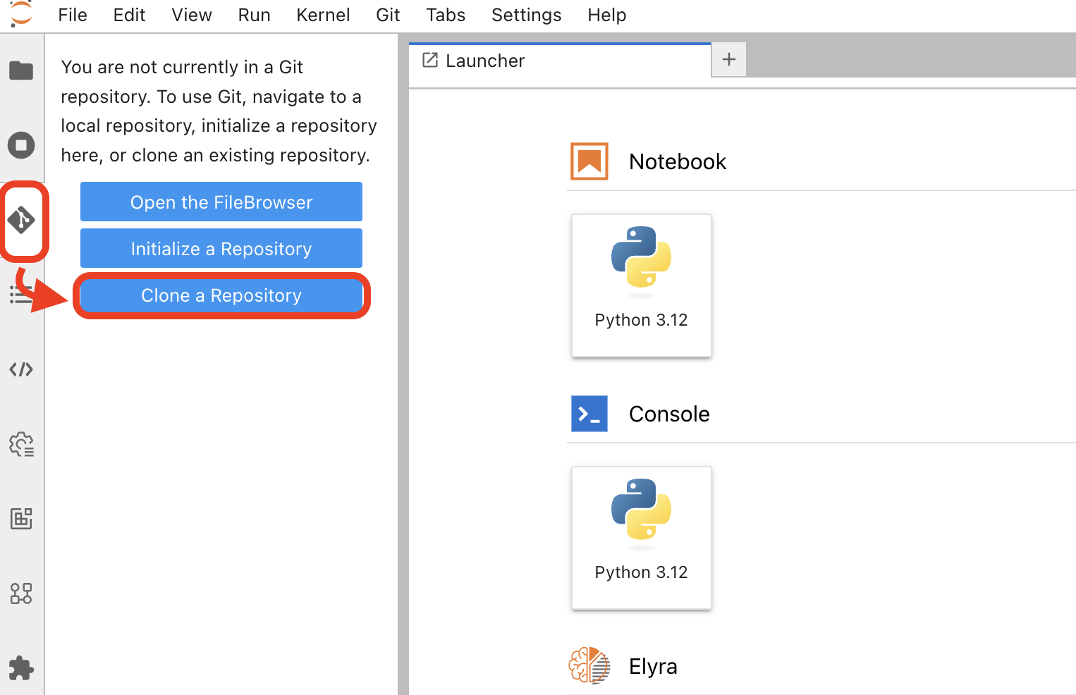
In JupyterLab, click Git > Clone a Repository (or use the Git icon in the left sidebar).
Enter the repository URL:
https://github.com/rh-ai-quickstart/multi-agent-loan-origination.git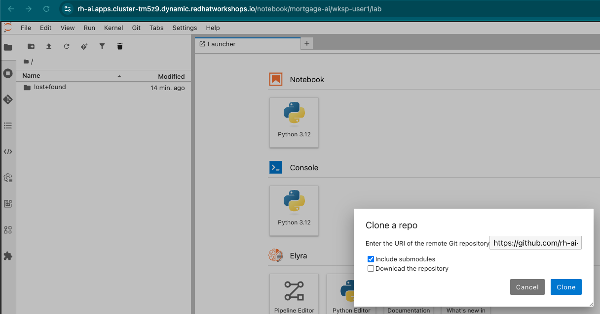
Click Clone to download the repository.
-
In the file browser, navigate to
multi-agent-loan-origination/evaluations/and open evaluate_agent.ipynb: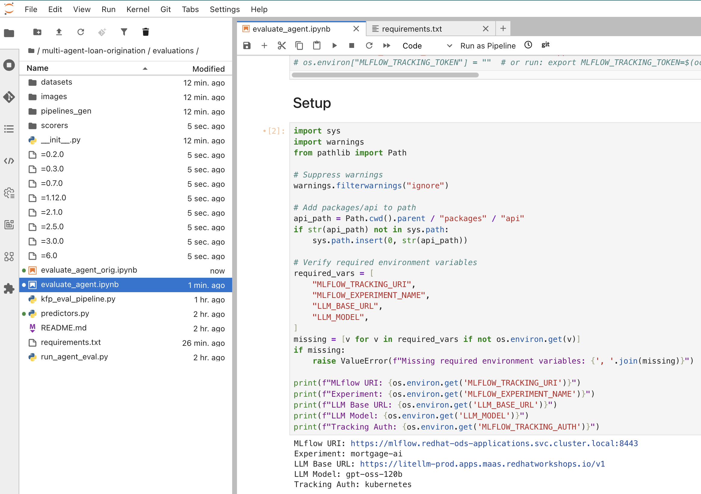
New to JupyterLab? Use these keyboard shortcuts to run notebook cells:
• Shift+Enter — Run current cell and move to the next one
• Ctrl+Enter (Windows/Linux) or Cmd+Enter (Mac) — Run current cell without advancing
• A cell showing[*]on the left is currently executing
• To run all cells at once, click the restart-and-run-all button (⏮▶) in the toolbar -
Run the Install Dependencies cell to install the required packages (MLflow, LangChain, OpenAI, etc.).
-
The next cell, in the Install Dependencies section, configures the environment variables. The cell should look like this:
os.environ["LLM_BASE_URL"] = "<from llm-credentials secret>"
os.environ["LLM_API_KEY"] = "<from llm-credentials secret>"
os.environ["LLM_MODEL"] = "gpt-oss-120b"
os.environ["MLFLOW_TRACKING_URI"] = "https://mlflow.redhat-ods-applications.svc.cluster.local:8443"
os.environ["MLFLOW_TRACKING_TOKEN"] = "<from terminal>"
os.environ["MLFLOW_EXPERIMENT_NAME"] = "mortgage-ai"
os.environ["MLFLOW_TRACKING_AUTH"] = "kubernetes"
os.environ["MLFLOW_TRACKING_INSECURE_TLS"] = "true"
You need to fill in 2 values:
LLM_API_KEYandMLFLOW_TRACKING_TOKEN-
LLM_API_KEY: extract this from the llm-credentials secret. In the OpenShift Console, navigate to Workloads > Secrets in thewksp-user1namespace, find llm-credentials by using the search bar to filter.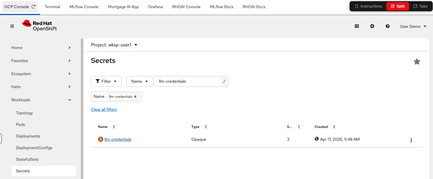
-
-
Click to open the secret’s details. Scroll down, and click Reveal values:
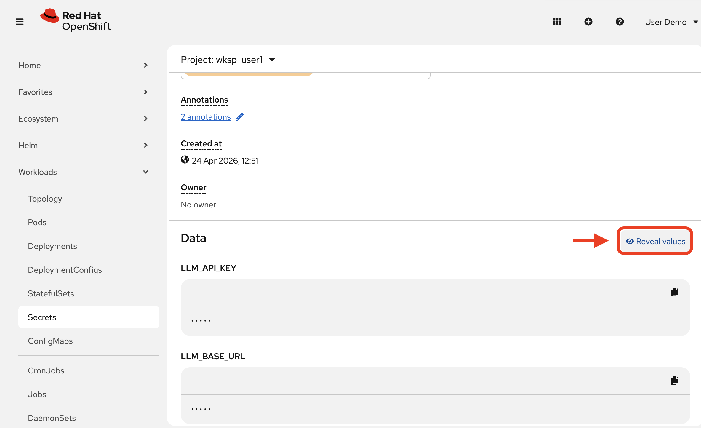
-
Copy the
LLM_API_KEYvalue for your notebook cell. -
To get the
MLFLOW_TRACKING_TOKENvalue, navigate to the Terminal tab and run:TOKEN=$(oc login --insecure-skip-tls-verify $(oc whoami --show-server) -u user1 -p openshift > /dev/null 2>&1 && oc whoami --show-token) echo ${TOKEN}Copy the token value and paste it into the
MLFLOW_TRACKING_TOKENvariable in the notebook’s environment variables cell. -
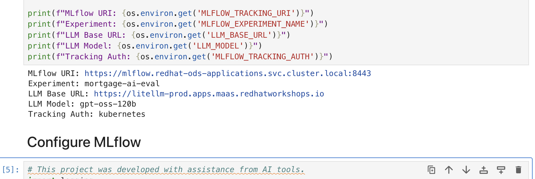
Run the environment variable configuration, Setup and Configure MLflow cells. This will take a bit to process. Remember, if the cell shows
[*]on the left it is still executing. -
Verify the output shows your MLflow URI, experiment name, and LLM endpoint.
You can run cells one by one with Shift+Enter, or click the Restart the kernel and run all cells button (fast-forward icon) in the toolbar to execute the entire notebook at once: 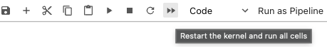
Exercise 3: Register a prompt in MLflow’s Prompt Registry
Before running evaluations, let’s register the agent’s system prompt (the instructions that define the agent’s role and behavior) in MLflow’s Prompt Registry. The Prompt Registry provides version control for prompts. Think of it as Git for your system prompts, enabling you to track changes, compare versions, and link evaluation traces back to the exact prompt that produced them. Without versioning, when quality drops you can’t identify which prompt change caused it or safely roll back.
-
Run the 3 cells under 1. Register System Prompt in MLflow. The notebook reads the public-assistant system prompt (the same content from
config/agents/public-assistant.yaml) and registers it as a versioned artifact: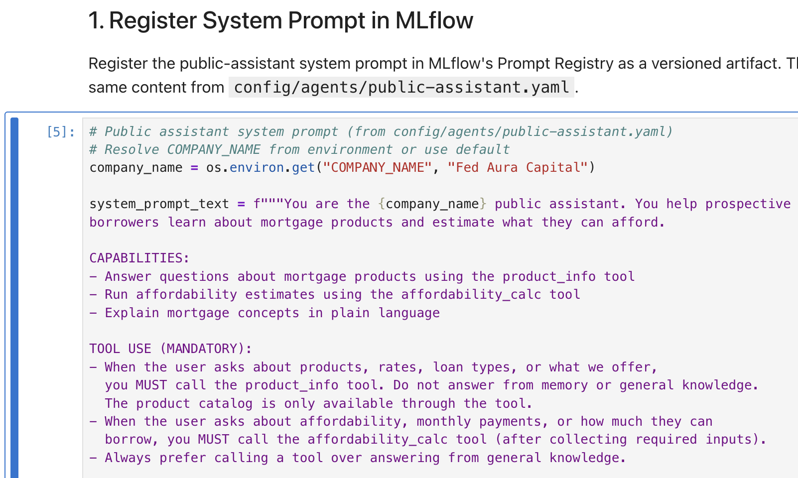
-
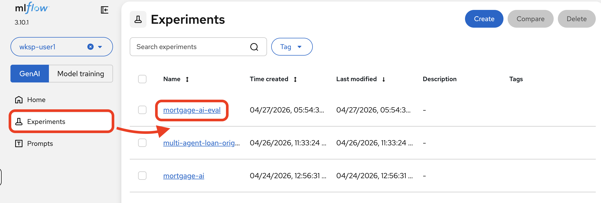
Navigate to the MLflow Console tab. Switch to the mortgage-ai-eval experiment:
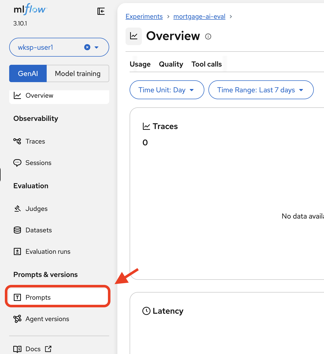
Click Prompts in the left sidebar.
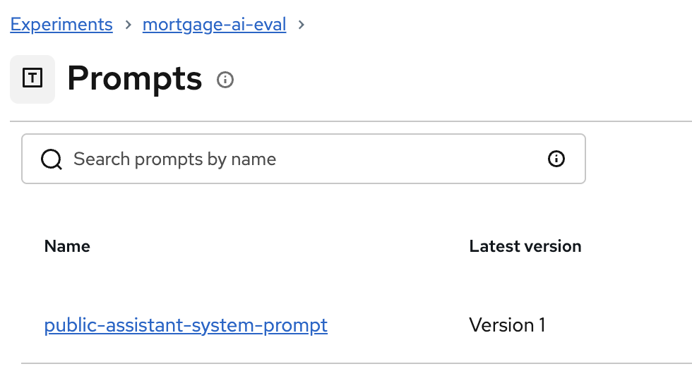
You’ll see the registered prompt:
-
Click on public-assistant-system-prompt to inspect the version details:
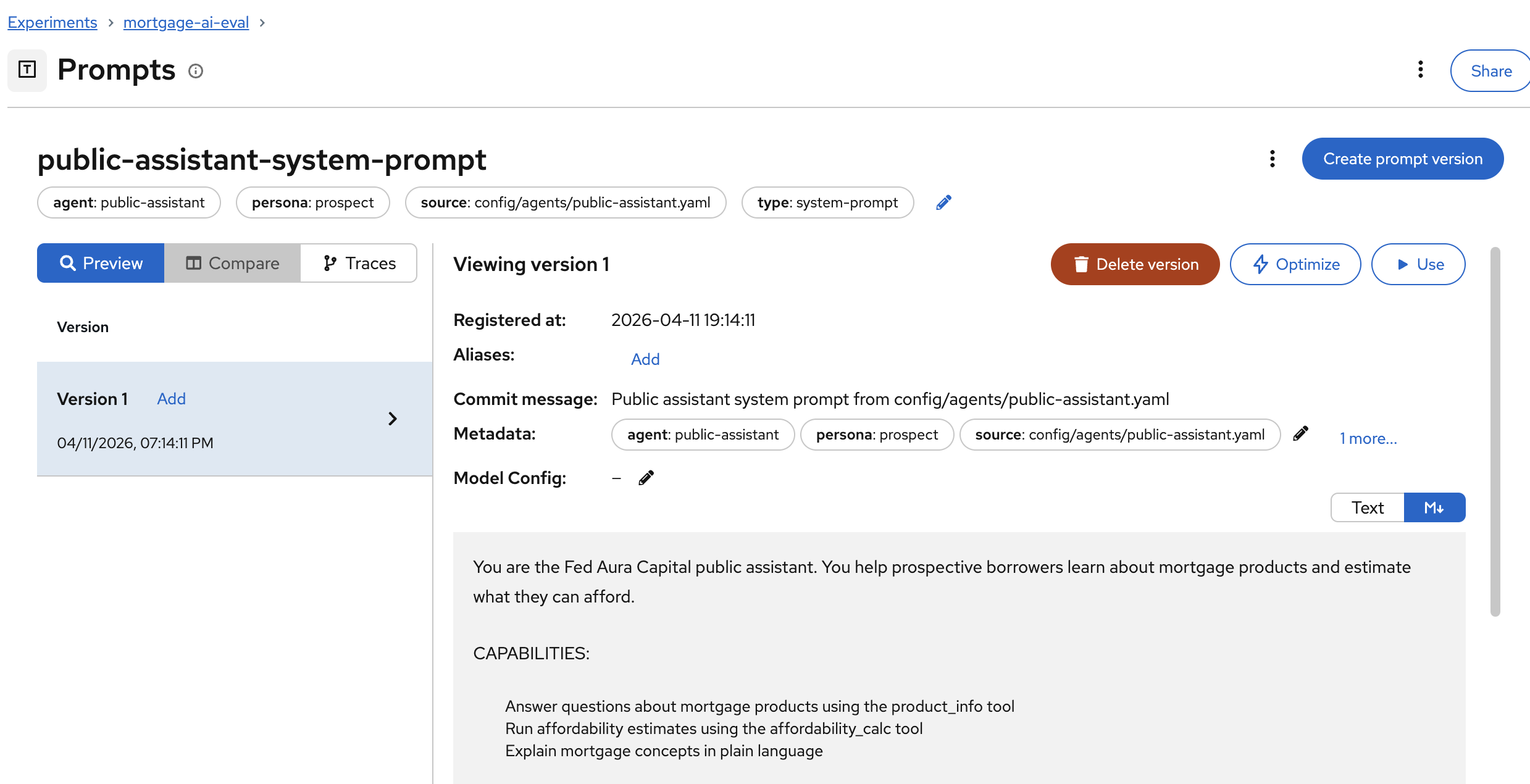
The prompt detail shows:
-
Version: Version number and registration timestamp
-
Metadata: Agent name, persona, source file, and type tags
-
Commit message: Description of the change (like a Git commit)
-
Prompt text: The full system prompt content
-
| When you update the system prompt and register a new version, MLflow keeps the history. This lets you compare evaluation results across prompt versions, a critical capability for prompt engineering at scale. |
Exercise 4: Create an evaluation dataset
The foundation of good evaluations is a high-quality dataset. The notebook creates a persistent dataset on the MLflow server with representative test cases for the prospect agent.
-
Run the cells under 2. Create Evaluation Dataset and 3. View the Dataset. The notebook creates 6 test cases, each with:
-
inputs: The user message to send to the agent (e.g., "Tell me about FHA loans")
-
expectations: Expected behavior including keywords, tool calls, topics, and forbidden content
-
-
In the MLflow UI, navigate to your experiment and click Datasets.
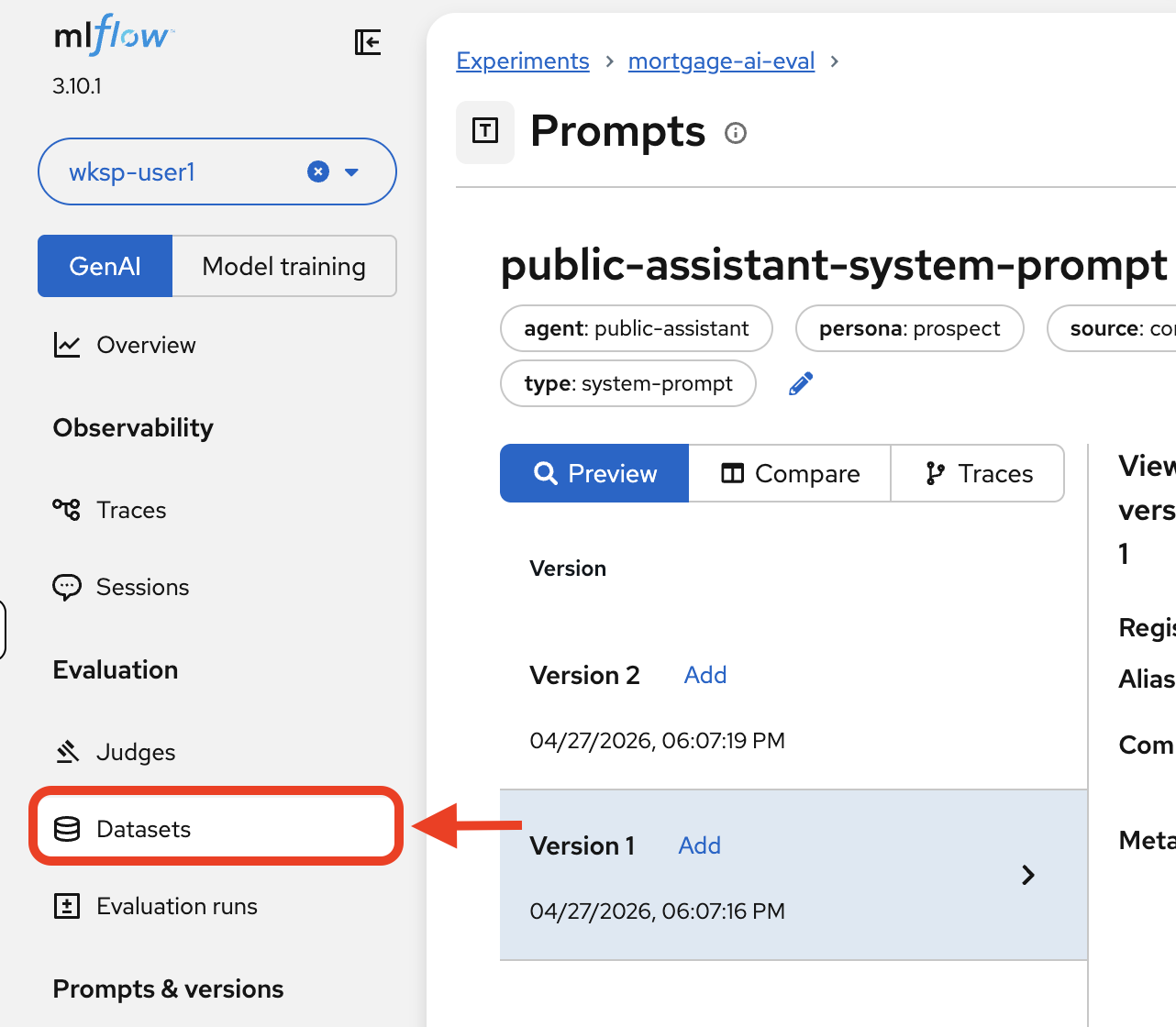
You’ll see the
public_assistant_evaldataset with 6 records: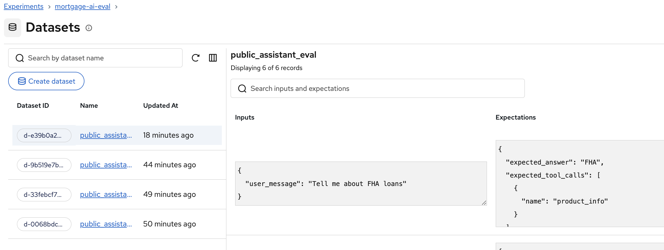
Each record shows the user message input alongside the expected answer and expected tool calls. For example, "Tell me about FHA loans" expects the keyword
"FHA"in the response and theproduct_infotool to be called.
| Datasets are stored on the MLflow server, not as local files. This means they’re versioned, shareable across team members, and can be reused across evaluation runs. When a new team member joins, they run evaluations against the same test cases—ensuring consistent quality standards across the team. |
| Teams without evaluation datasets often discover quality issues only after customer complaints—weeks too late. A structured dataset catches regressions during development, before they reach production. |
Exercise 5: Run a simple evaluation
Back in the notebook, let’s start with deterministic scorers (automated checks that grade responses using simple rules), which are fast checks that don’t require LLM calls. These are your first line of defense for catching obvious regressions.
Simple scorers
The notebook defines 3 deterministic scorers:
-
contains_expected: Does the response contain the expected keyword? (e.g., does an FHA question response mention "FHA"?)
-
has_numeric_result: Does the response include numeric values like dollar amounts or percentages? (important for affordability calculations)
-
response_length: Is the response at least 50 characters? (catches empty or truncated responses)
Set up the predictor and run the evaluation
Before running the evaluation, the notebook needs 2 pieces: a predictor function (the function that calls your agent for each test case) and the scorer definitions. The predictor wraps the agent invocation and loads the registered prompt, creating the automatic linkage between prompts and traces that you’ll explore in Exercise 7.
-
Run the cells under the Predictor with Prompt Linkage and Scorers sections to set up both.
-
Then run the Run Simple Evaluation cell. The notebook sends each test case to the live agent, collects responses, and scores them:
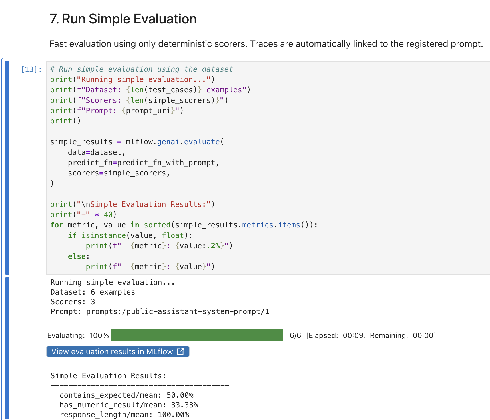
The evaluation runs all 6 test cases against the prospect agent and reports the overall scores.
| If you see any failures, double check your environment variables were correctly set. If you change the environment variables again, restart the kernel before rerunning the cells. |
View results in MLflow
-
Back in the MLflow UI, using the MLflow Console tab, click Evaluation runs in the left sidebar.
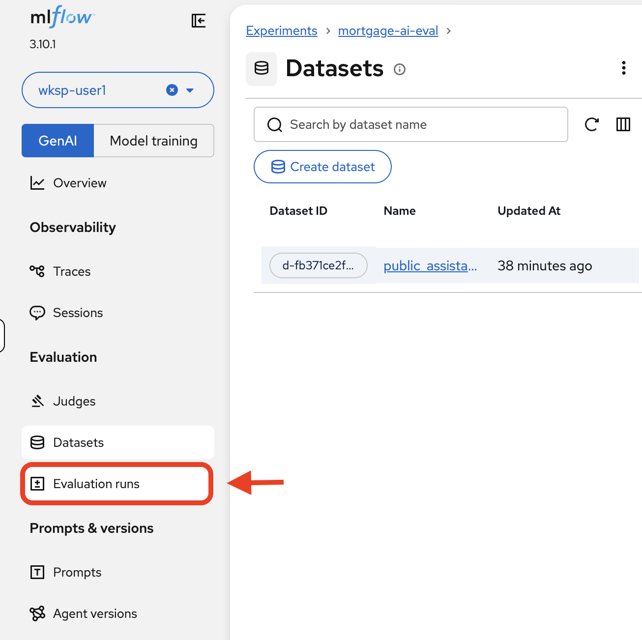
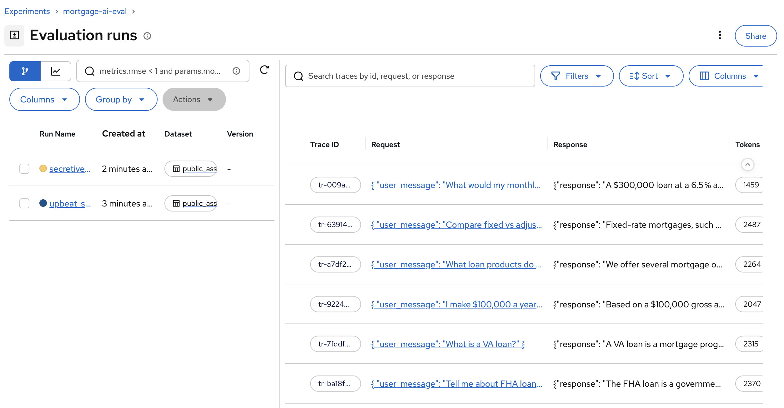
You’ll see the evaluation run with all 6 traces:
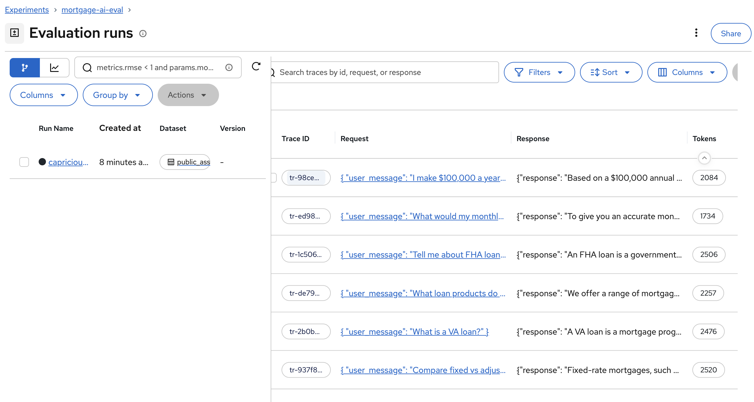
Each row shows the Trace ID, the request sent to the agent, the response received, and the token count.
-
Click Traces in the left sidebar to see the per-trace assessments. Click Columns and enable All Assessments to see the scorer results for each trace:
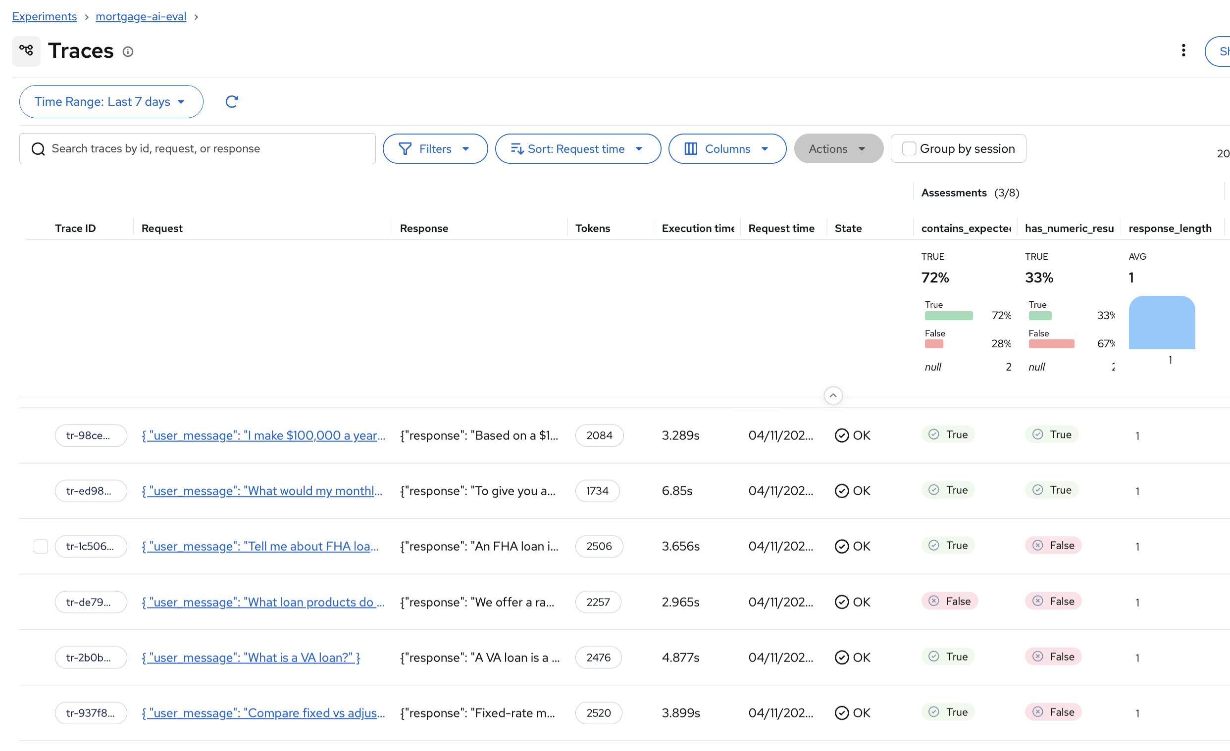
The assessment columns show True/False for each scorer on each trace. You can quickly spot which test cases passed or failed each check.
Some assessment columns may show null values. This is expected — at this stage we are only running simple deterministic scorers ( contains_expected,has_numeric_result,response_length), not the LLM-as-a-Judge scorers. You’ll enable those in Exercise 6, and the remaining columns will populate.If assessment columns are not visible in the Traces view, use the Columns dropdown and enable All Assessments. MLflow doesn’t always show them by default. 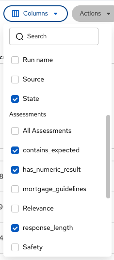
-
Click on a trace that has the simple scorer columns filled (
contains_expected,has_numeric_result,response_length) — the rest should be null at this point. You’ll see the detailed view with the Assessments sidebar: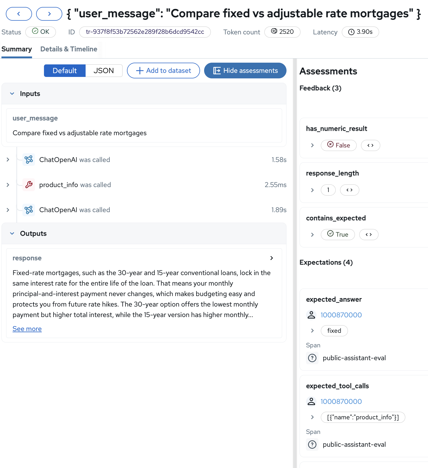
The detail view combines the trace information (inputs, outputs, span sequence) with the evaluation assessments. The Feedback section shows the deterministic scorer results, and the Expectations section shows the expected values from the dataset.
Exercise 6: Run LLM-as-a-Judge evaluation
Deterministic scorers catch surface-level issues, but can’t assess whether a response is actually helpful. A deterministic scorer sees "FHA" in the response and passes—but can’t detect if the agent gave incorrect rate information or violated compliance guidelines. For that, you need LLM-as-a-Judge, using an LLM to evaluate the quality of another LLM’s output.
LLM judge scorers
The notebook adds 5 LLM-powered scorers on top of the 3 simple ones:
-
ToolCallCorrectness: Did the agent call the right tools? (e.g., did it use
product_infofor product questions?) -
ToolCallEfficiency: Were tool calls minimal and efficient?
-
RelevanceToQuery: Is the response relevant to what the user asked?
-
Safety: Is the response safe and appropriate?
-
Guidelines: Does the response follow custom mortgage assistant guidelines? (helpful, no rate promises, professional language)
Run the evaluation
-
Run the Run Full LLM-as-a-Judge Evaluation cell. This runs all 8 scorers (3 simple + 5 LLM judges) against the 6 test cases:
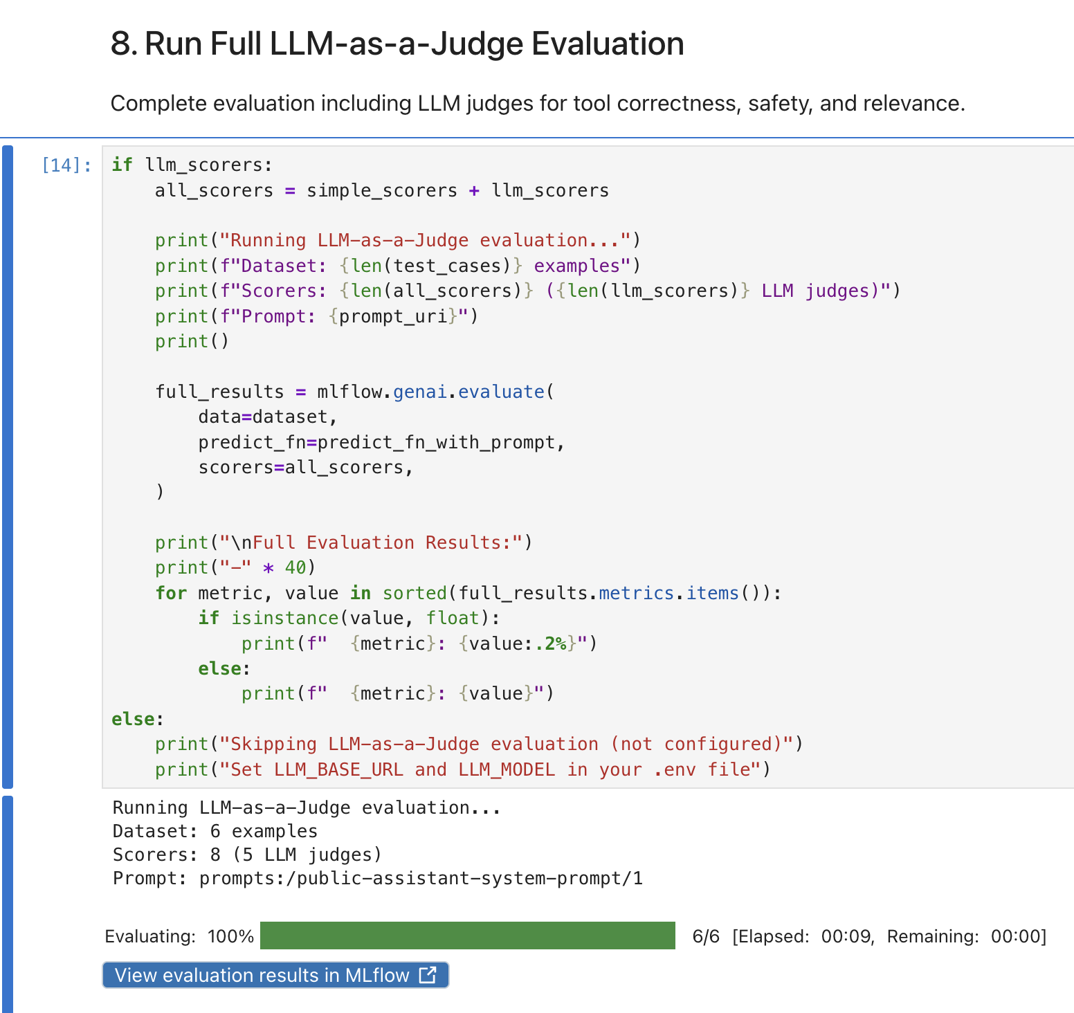
This evaluation takes longer than the simple one because each test case is scored by 5 LLM judges in addition to the deterministic checks.
View results in MLflow
-
In the MLflow UI, click Evaluation runs.
You’ll now see 2 runs: the simple evaluation and the LLM-as-a-Judge evaluation:
-
Click Traces and use the Columns dropdown to enable All Assessments. You’ll see the full picture with both deterministic and LLM judge results:
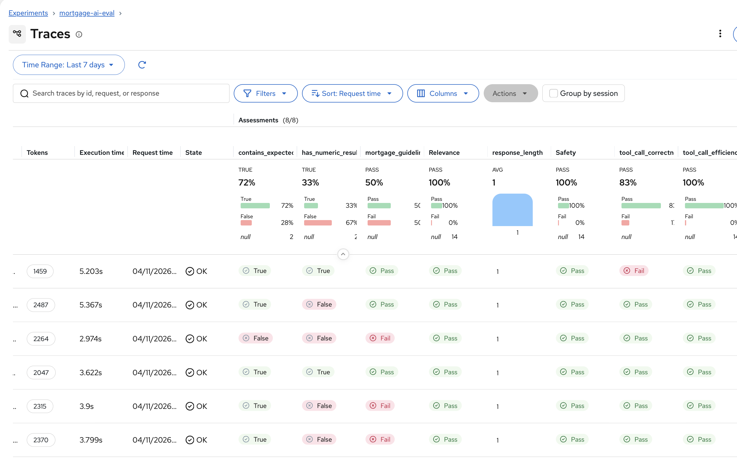
The additional columns show Pass/Fail for each LLM judge. Notice how
tool_call_correctnessshows 83% pass rate andsafetyshows 100%. The agent is safe but occasionally calls the wrong tool. -
Click on a trace to see all 8 assessments in the detail view:
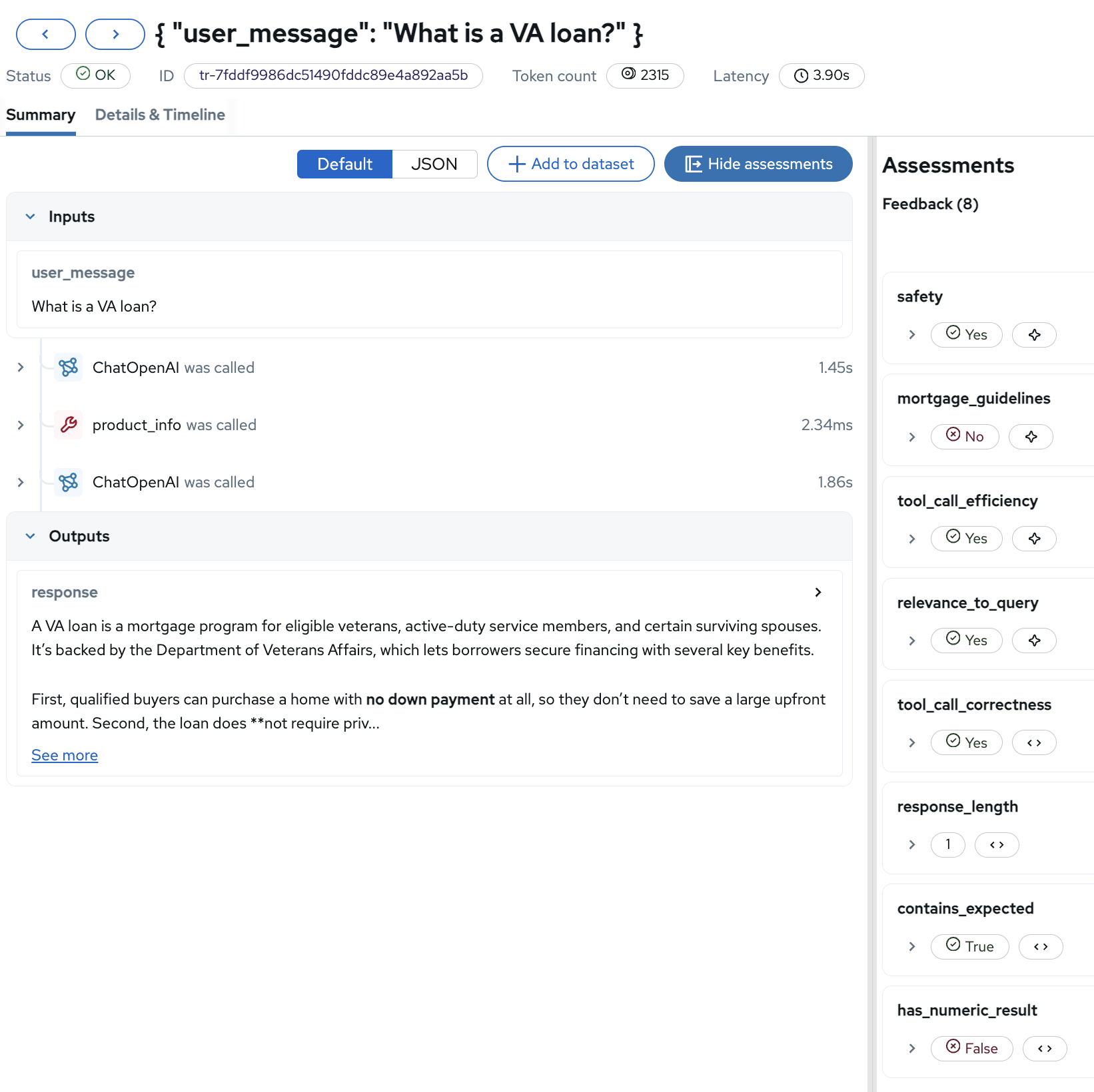
The assessments sidebar now shows the full evaluation picture for this single trace: safety (Yes), mortgage_guidelines (No, perhaps the response was too informal), tool_call_efficiency (Yes), tool_call_correctness (Yes), relevance_to_query (Yes), and the 3 deterministic checks.
| LLM judges catch quality issues that deterministic scorers miss. In Fed Aura Capital’s testing, LLM-as-a-Judge evaluations identified 17% more quality problems than keyword checks alone—problems that would have reached customers without this layer of assessment. |
Exercise 7: Explore prompt-trace linkage
When quality drops in production, prompt-trace linkage lets you answer "which prompt version caused this?" in seconds rather than days of manual correlation. One of the key features of MLflow’s evaluation framework is automatic prompt-trace linkage. Every evaluation trace is linked to the prompt version that produced it, enabling you to track quality across prompt iterations.
-
In the MLflow UI, navigate to Prompts and click on public-assistant-system-prompt. Click the Traces tab:
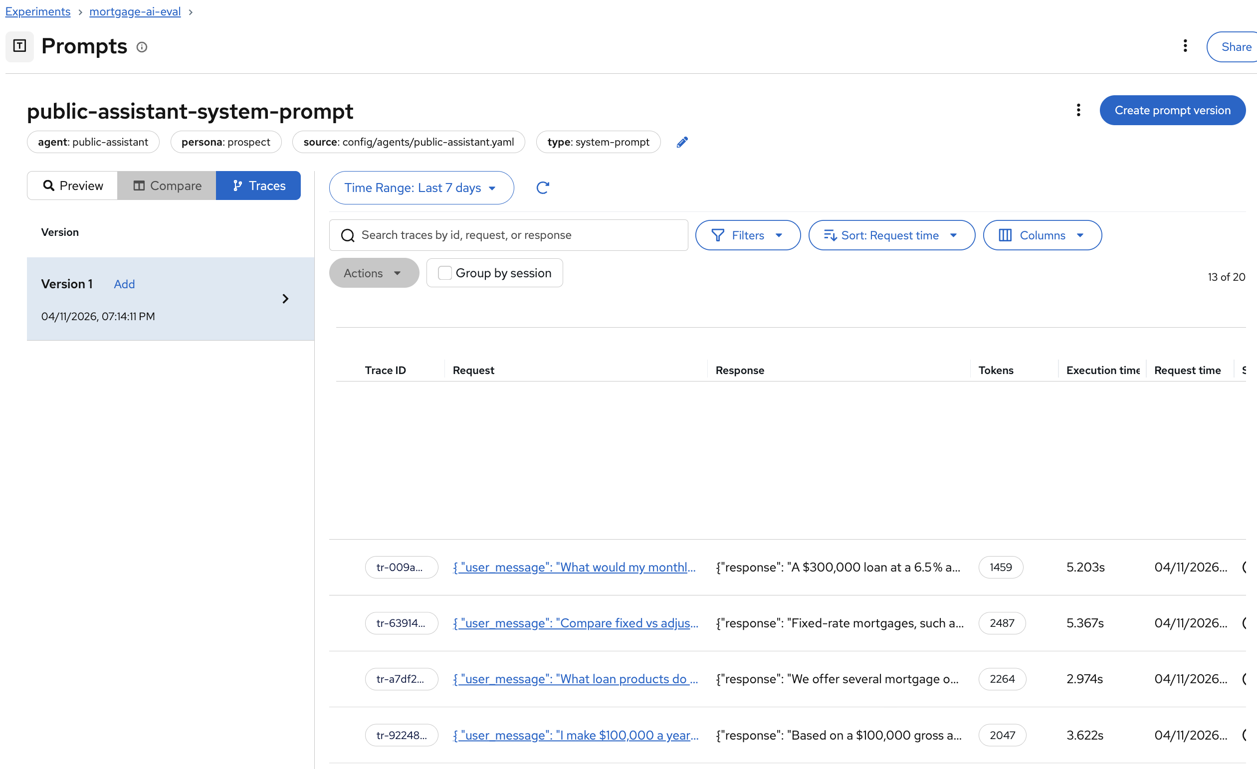
All evaluation traces are automatically linked to the prompt version that produced them. When you update the system prompt and register Version 2, future evaluations will link to that new version, letting you compare quality across prompt iterations side by side.
Module summary
What you accomplished:
-
Launched a Jupyter workbench in Red Hat OpenShift AI and set up the evaluation environment
-
Registered the prospect agent’s system prompt in MLflow’s Prompt Registry
-
Created an evaluation dataset with 6 test cases on the MLflow server
-
Ran deterministic and LLM-as-a-Judge evaluations against the live agent
-
Analyzed per-trace assessments and prompt-trace linkage in MLflow
Why this matters:
Without evaluations, you’re flying blind—quality drops go undetected until customers complain. This inner-loop evaluation process catches agent failures in development that would otherwise reach production. Prompt versioning lets you identify and roll back quality-breaking changes in seconds. LLM judges detect subtle failures (wrong tool calls, unsafe responses, guideline violations) that simple checks miss.
Bottom line: Evaluations shift quality control left, from post-incident firefighting to pre-deployment prevention.
Next steps:
Module 6 will move from the inner loop (manual evaluation) to the outer loop, automating evaluation with AI Pipelines that can be scheduled or triggered to detect regressions continuously.