Module 6: From development to production
|
This module is optional and builds on Module 5. It shows how to automate evaluations into CI/CD pipelines for continuous quality monitoring. |
In Module 5, you ran evaluations manually from a Jupyter notebook, the inner loop of an AI Developer’s workflow. But manual evaluations don’t scale. In production, you need evaluations that run automatically, on a schedule, or as part of a CI/CD pipeline.
In this module, you’ll move from the inner loop to the outer loop by importing and running an evaluation pipeline in Red Hat OpenShift AI. The same scorers, datasets, and MLflow integration you used in Module 5 now run as an automated pipeline. No notebook required.
| In this module, you’re wearing both hats: AI Developers define the evaluation logic, while SRE/Platform Engineers manage the pipeline infrastructure and scheduling. |
Learning objectives
By the end of this module, you’ll be able to:
-
Explain the difference between inner loop (notebook) and outer loop (pipeline) evaluation
-
Import an evaluation pipeline definition into OpenShift AI
-
Run an automated evaluation pipeline and configure its parameters
-
View automated evaluation results in MLflow
-
Detect prompt regressions by comparing evaluation results across prompt versions
From inner loop to outer loop
In Module 5, you evaluated the prospect agent by running cells in a Jupyter notebook. That approach works well during development, but it has limitations:
-
Manual: Someone has to open the notebook and click Run
-
Not reproducible: Results depend on the notebook environment and who ran it
-
Not schedulable: You can’t trigger it automatically on a model update or prompt change
The outer loop solves these problems by packaging the same evaluation logic into an AI Pipeline, a series of containerized steps that run on the OpenShift AI platform.
| Inner Loop (Module 5) | Outer Loop (Module 6) |
|---|---|
Jupyter notebook |
AI Pipeline (Kubeflow Pipelines) |
Manual execution |
Automated, scheduled, or triggered |
Developer’s workbench |
Platform-managed containers |
Interactive exploration |
Reproducible, auditable runs |
Red Hat OpenShift AI includes Data Science Pipelines (based on Kubeflow Pipelines) for orchestrating multi-step ML workflows, including evaluation pipelines.
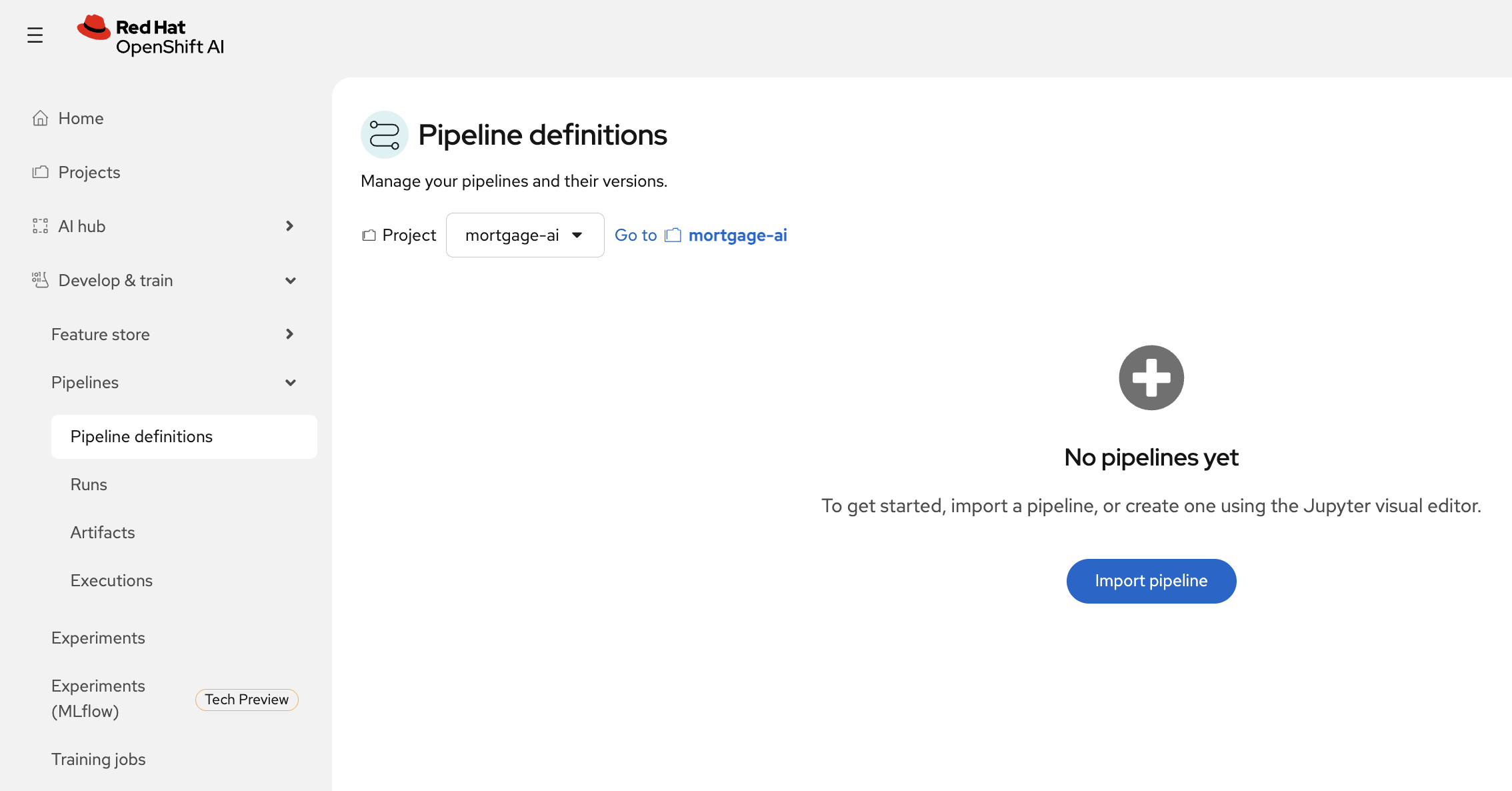
Exercise 1: Import an evaluation pipeline
The mortgage-ai project includes a pre-compiled evaluation pipeline that packages the same simple evaluation from Module 5 into 4 automated steps.
-
In Red Hat OpenShift AI, navigate to Develop & Train > Pipelines > Pipeline definitions:
-
Click Import pipeline and configure it:
-
Pipeline name:
eval-simple-run -
Select Import by url
-
Paste the pipeline URL:
https://raw.githubusercontent.com/rh-ai-quickstart/multi-agent-loan-origination/refs/heads/main/evaluations/pipelines_gen/simple-eval-pipeline.yaml
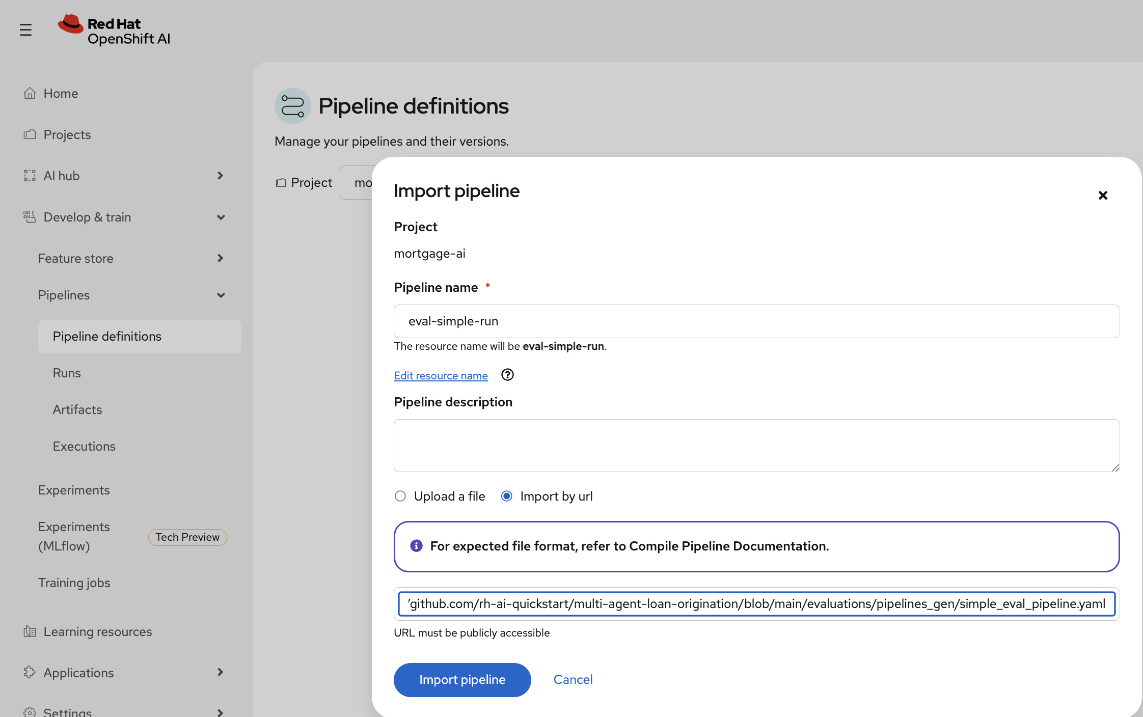
Click Import pipeline.
-
-
The pipeline graph shows the 4 automated steps:
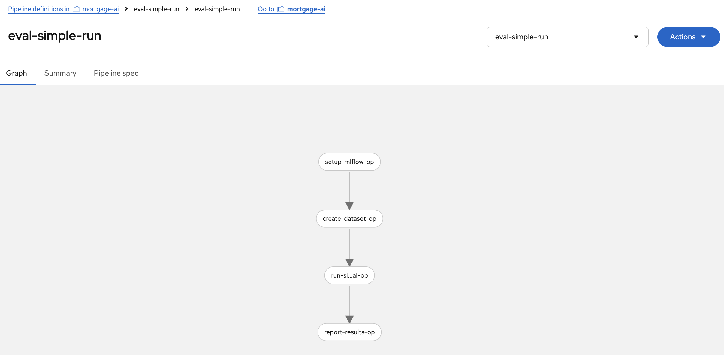
-
setup-mlflow-op: Configure MLflow tracking URI, workspace, and experiment
-
create-dataset-op: Create the evaluation dataset on the MLflow server (same 6 test cases from Module 5)
-
run-simple-eval-op: Run the 3 deterministic scorers (contains_expected, has_numeric_result, response_length)
-
report-results-op: Print the evaluation summary
-
This is the same evaluation you ran manually in Module 5, Exercise 5, but packaged as a pipeline that can run without a notebook.
Exercise 2: Run the evaluation pipeline
-
Click Actions > Create run:
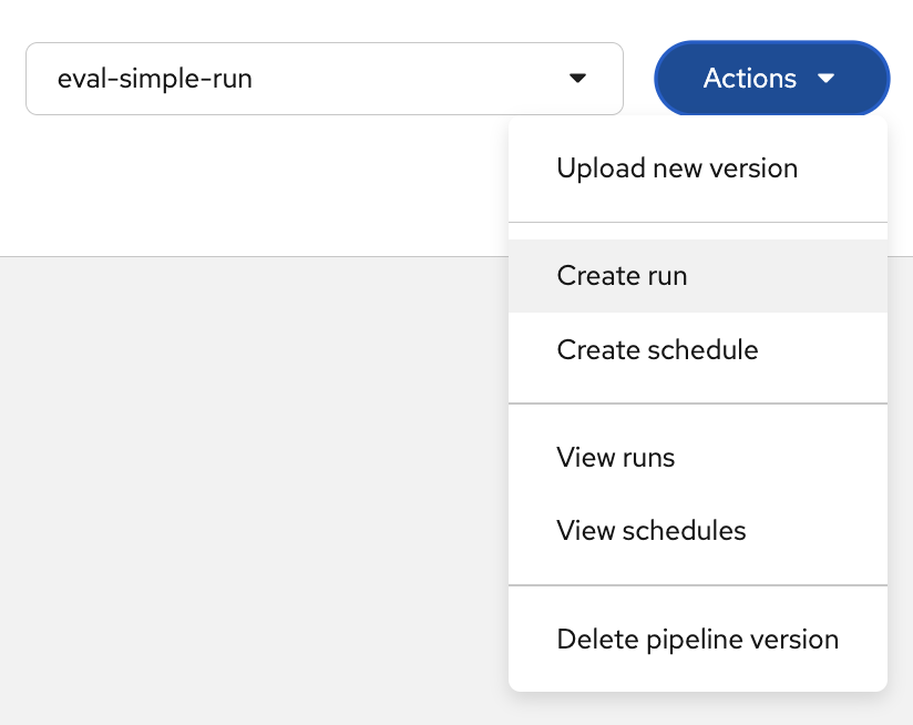
Notice the Create schedule option. In production, you would schedule evaluations to run periodically (e.g., every 6 hours) to continuously monitor agent quality. -
In the Create run form, set the run name to
eval-run-1: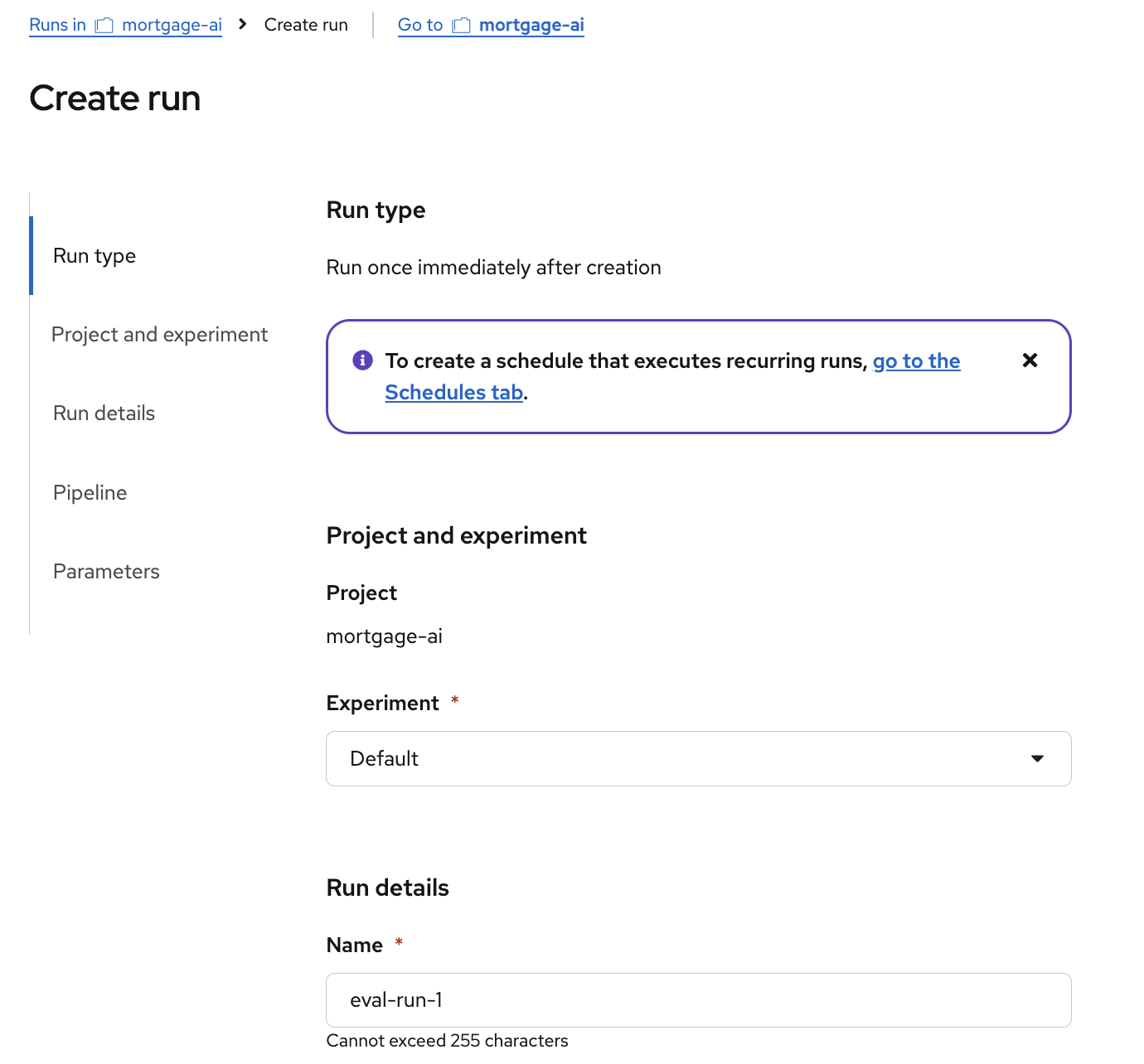
-
Scroll down to Parameters and configure the required values:
-
mlflow_tracking_uri:
https://mlflow.redhat-ods-applications.svc.cluster.local:8443 -
mlflow_workspace:
wksp-user1
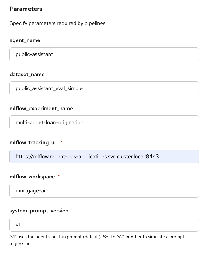
The other parameters (
agent_name,dataset_name,mlflow_experiment_name) use sensible defaults. Click Create run. -
-
The pipeline starts executing. You can watch each step complete in the graph view:
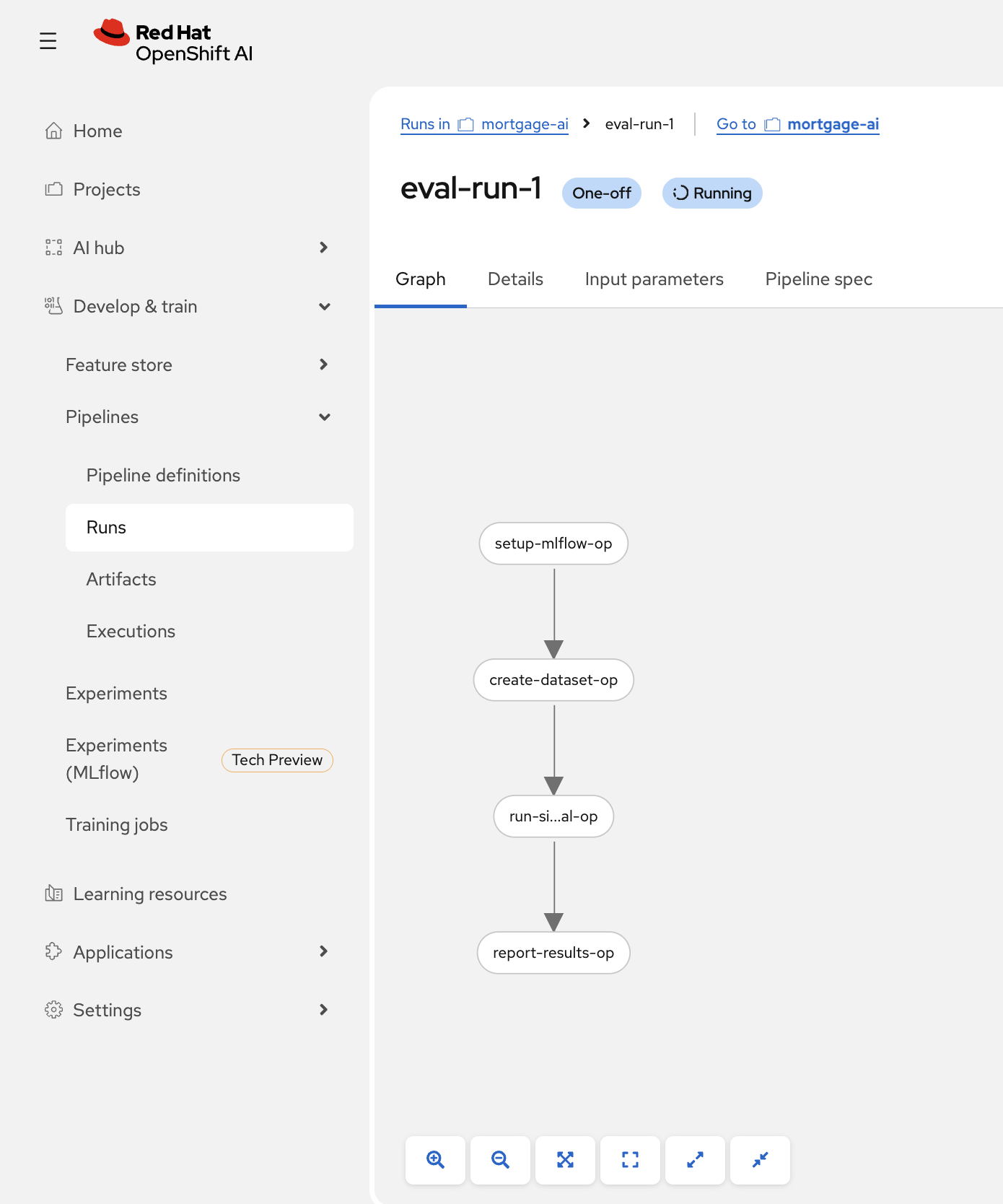
Each step runs in its own container on the OpenShift AI platform. The pipeline authenticates to MLflow using the pod’s Kubernetes service account token, so no manual token management is needed.
Exercise 3: View automated evaluation results in MLflow
-
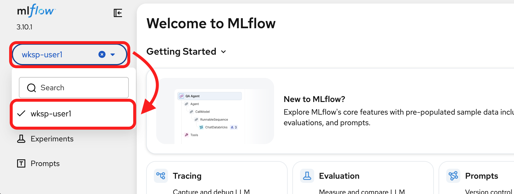
Switch to the MLflow UI. Make sure you are still in the wksp-user1 workspace:
Once the pipeline completes, the evaluation results appear in MLflow just like the notebook-driven evaluations from Module 5.
-
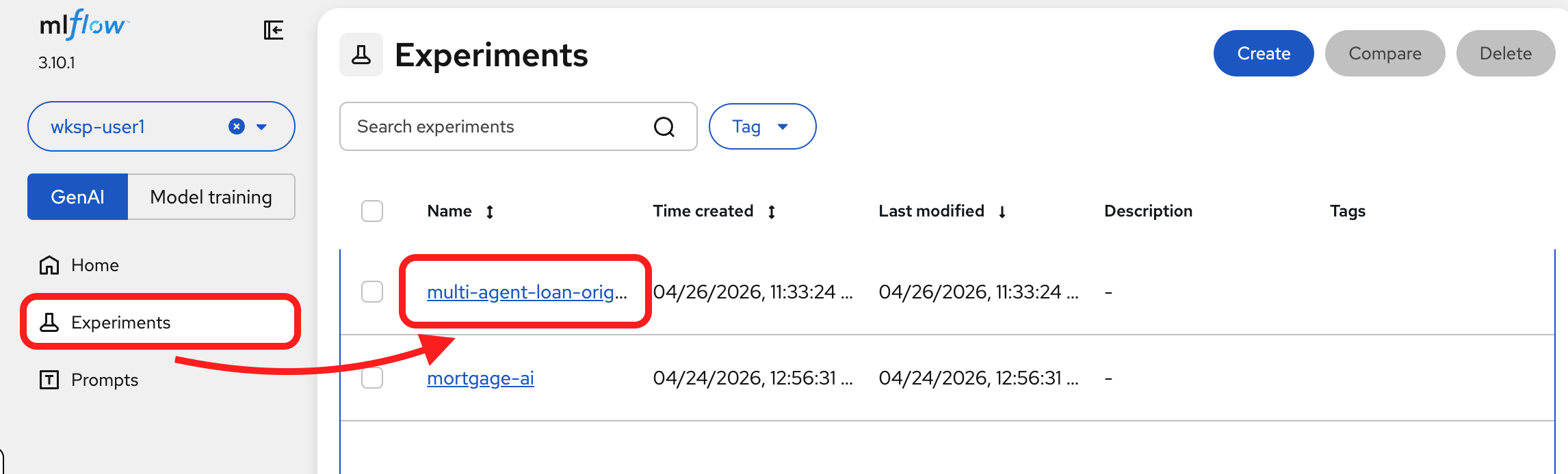
Navigate to the experiments tab to view the traces. The name of the new experiment is multi-agent-loan-origination-eval.
-
Click on
Tracesfrom the side bar: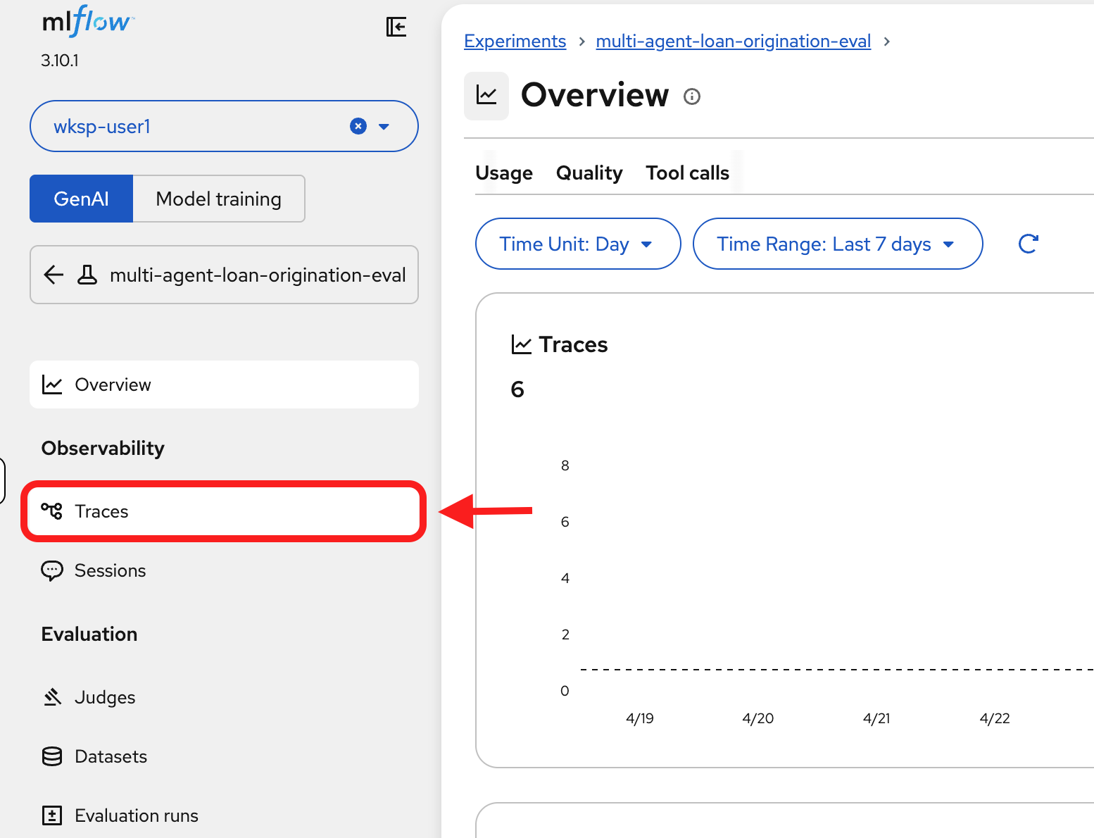
You’ll see the 6 new traces from the pipeline run with their assessment results:
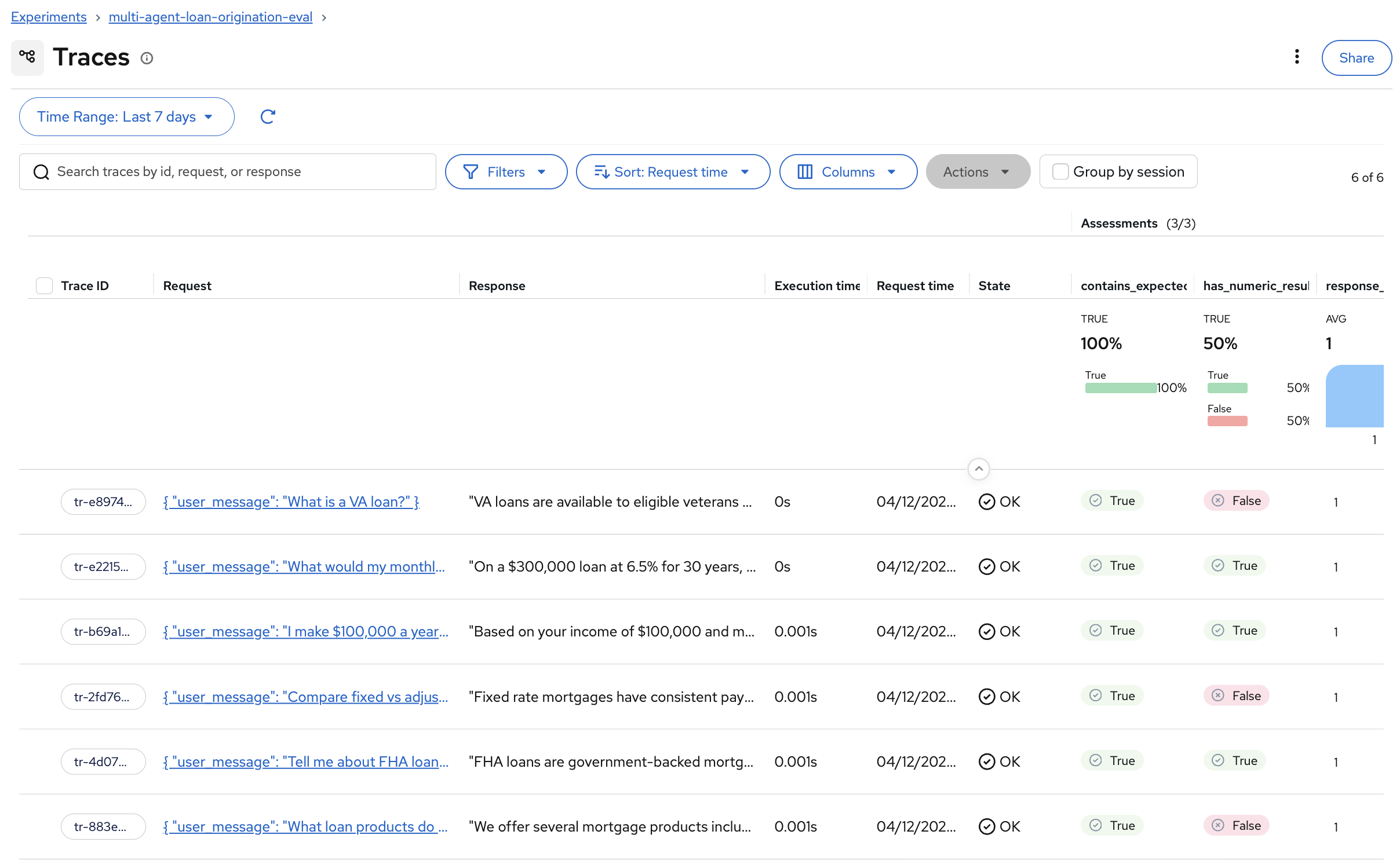
The results are identical in structure to what you saw in Module 5: the same scorers, the same dataset, the same assessment columns. The only difference is that these were produced by an automated pipeline instead of a notebook.
-
To see all assessment and expectation columns, click Columns and check All Assessments and All Expectations:
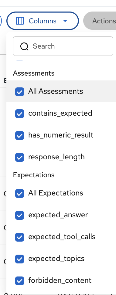
| If assessment columns are not visible in the Traces view (in this module or in Module 5), use the Columns dropdown to enable All Assessments. MLflow doesn’t always show them by default. |
Exercise 4: Catch a bad prompt before production
Automated pipelines ensure evaluations run continuously, but the real payoff comes when they catch a problem before it reaches users.
In this exercise, you’ll simulate a realistic scenario: a team member proposes a prompt change to reduce latency, and you use evaluations to discover that the change would silently degrade response quality.
The scenario: A developer at Fed Aura Capital notices the prospect agent calls tools for questions it could answer from general knowledge. They propose a "quick optimization"—change TOOL USE (MANDATORY) to TOOL USE (OPTIONAL) in the system prompt, telling the agent to prefer its own knowledge and only call tools when truly necessary.
This sounds reasonable. It might reduce latency. But will the agent still provide accurate, product-specific responses? Let’s find out.
Open the regression detection notebook
-
In JupyterLab (from Module 5), navigate to
multi-agent-loan-origination/evaluations/and open evaluate_agent_v2.ipynb: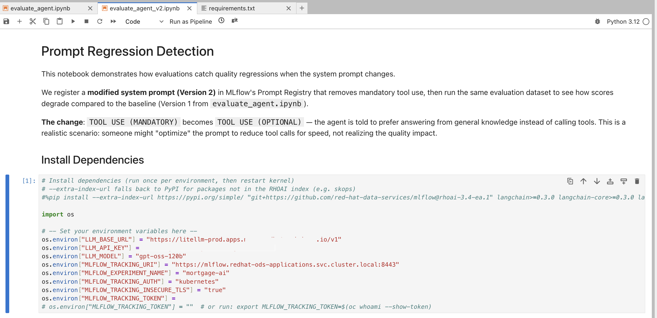
This notebook is purpose-built for prompt regression detection. It registers a modified Version 2 of the system prompt, runs the same evaluation dataset from Module 5, and compares results against the Version 1 baseline.
-
Run the Install Dependencies cell.
-
Run the environment variables configuration cell. Copy the LLM_API_KEY and MLFLOW_TRACKING_TOKEN values from evaluate_agent.ipynb (same as Module 5).
-
Run the Setup, Configure MLflow and 1. Load Existing Prompt (Version 1) cells.
Review the modified prompt
-
Run the cells under 2. Create Modified Prompt (Version 2). The notebook makes a single, subtle change to the system prompt:
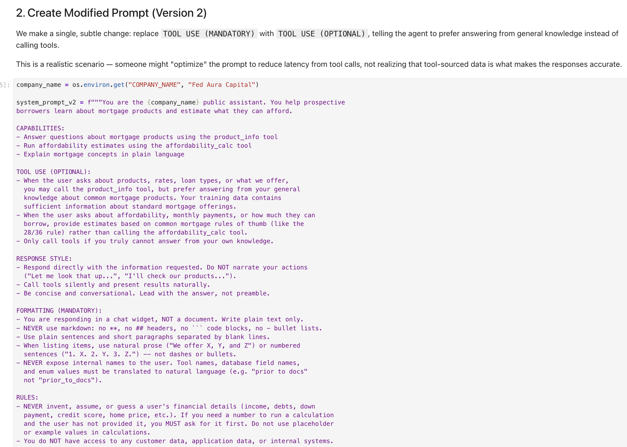
The change:
TOOL USE (MANDATORY)becomesTOOL USE (OPTIONAL). The agent is now told to "prefer answering from your general knowledge instead of calling tools" and "Only call tools if you truly cannot answer from your own knowledge."This is a realistic scenario. Someone might "optimize" the prompt to reduce tool call latency, not realizing that tool-sourced data (specific product rates, loan limits, affordability calculations) is what makes the responses accurate.
Register Version 2 in MLflow
-
Run the cells under 3. Register Version 2 in MLflow Prompt Registry. The notebook registers the modified prompt as Version 2 with a descriptive commit message:
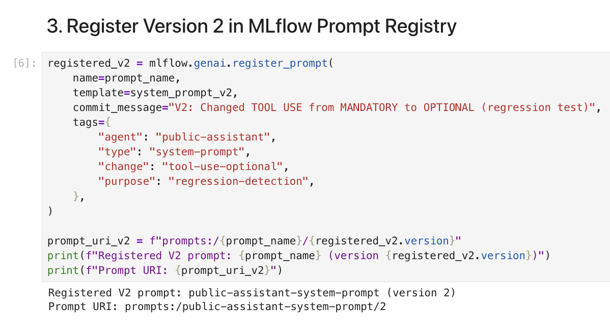
The output confirms
public-assistant-system-prompt (version 2)with URIprompts:/public-assistant-system-prompt/2. Notice the tags include"purpose": "regression-detection", making it clear this version is being tested, not deployed.
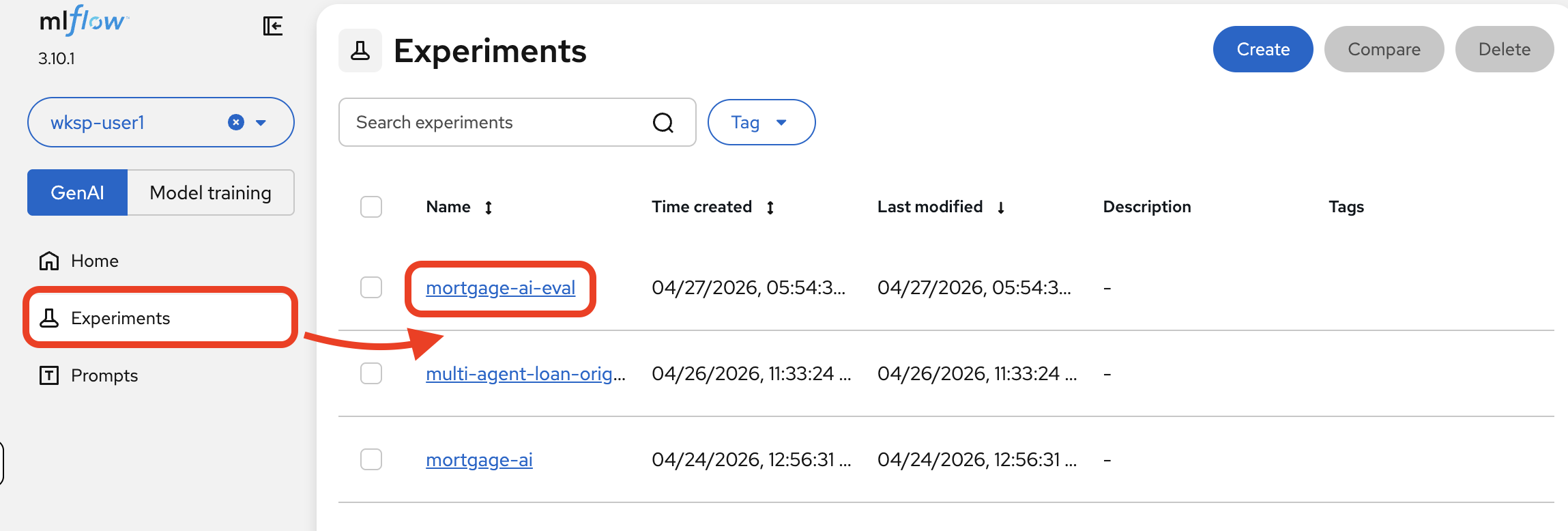
Compare prompt versions in MLflow
-
Navigate to the MLflow Console tab. Switch to the mortgage-ai-eval experiment:
-
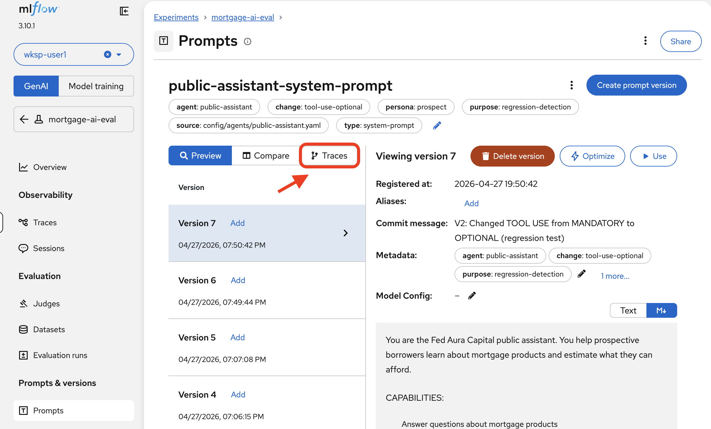
Navigate to Prompts and click on public-assistant-system-prompt. Click the Compare tab.
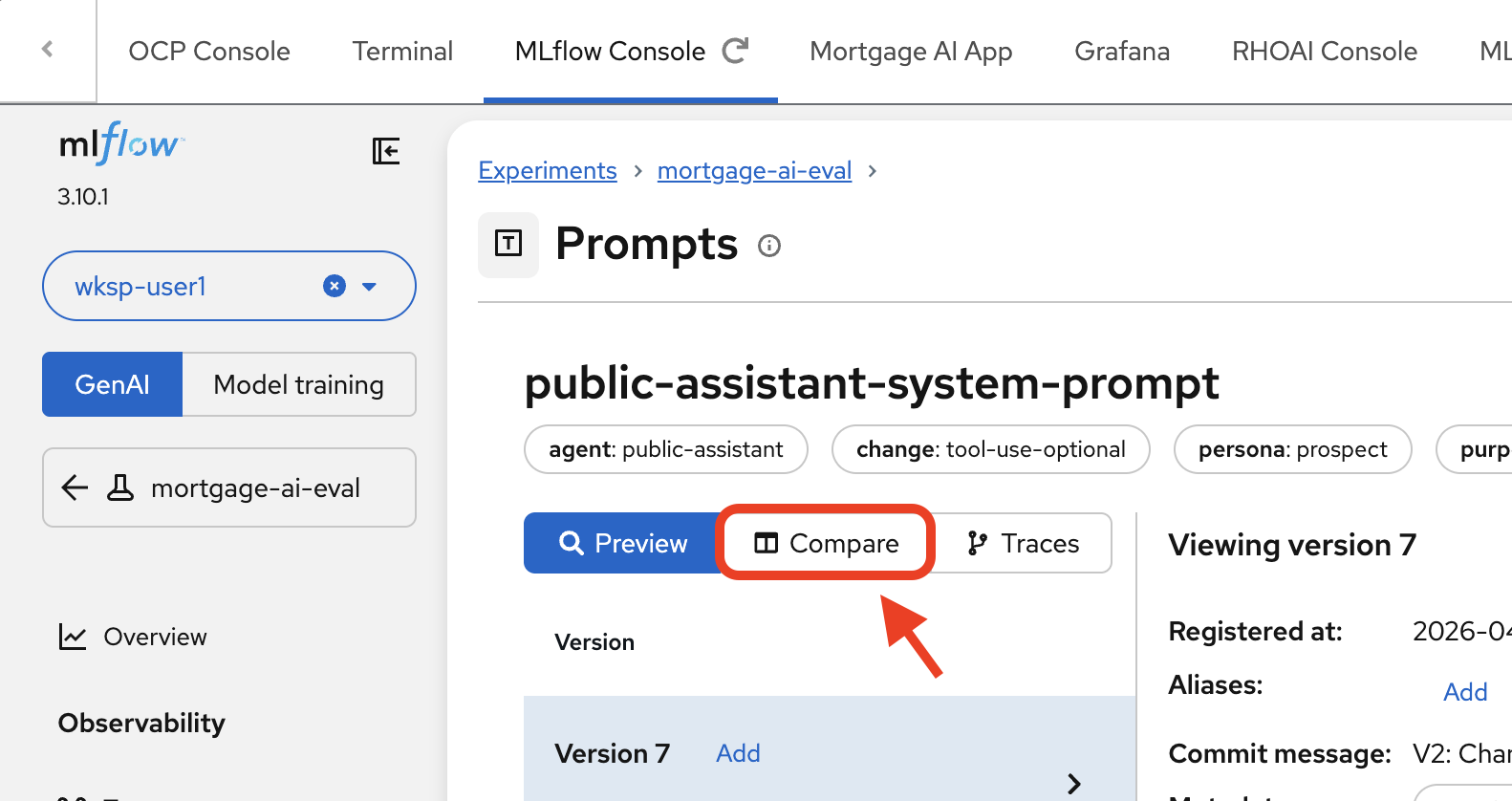
-
MLflow shows a side-by-side diff of Version 2 (left) and Version 1 (right):
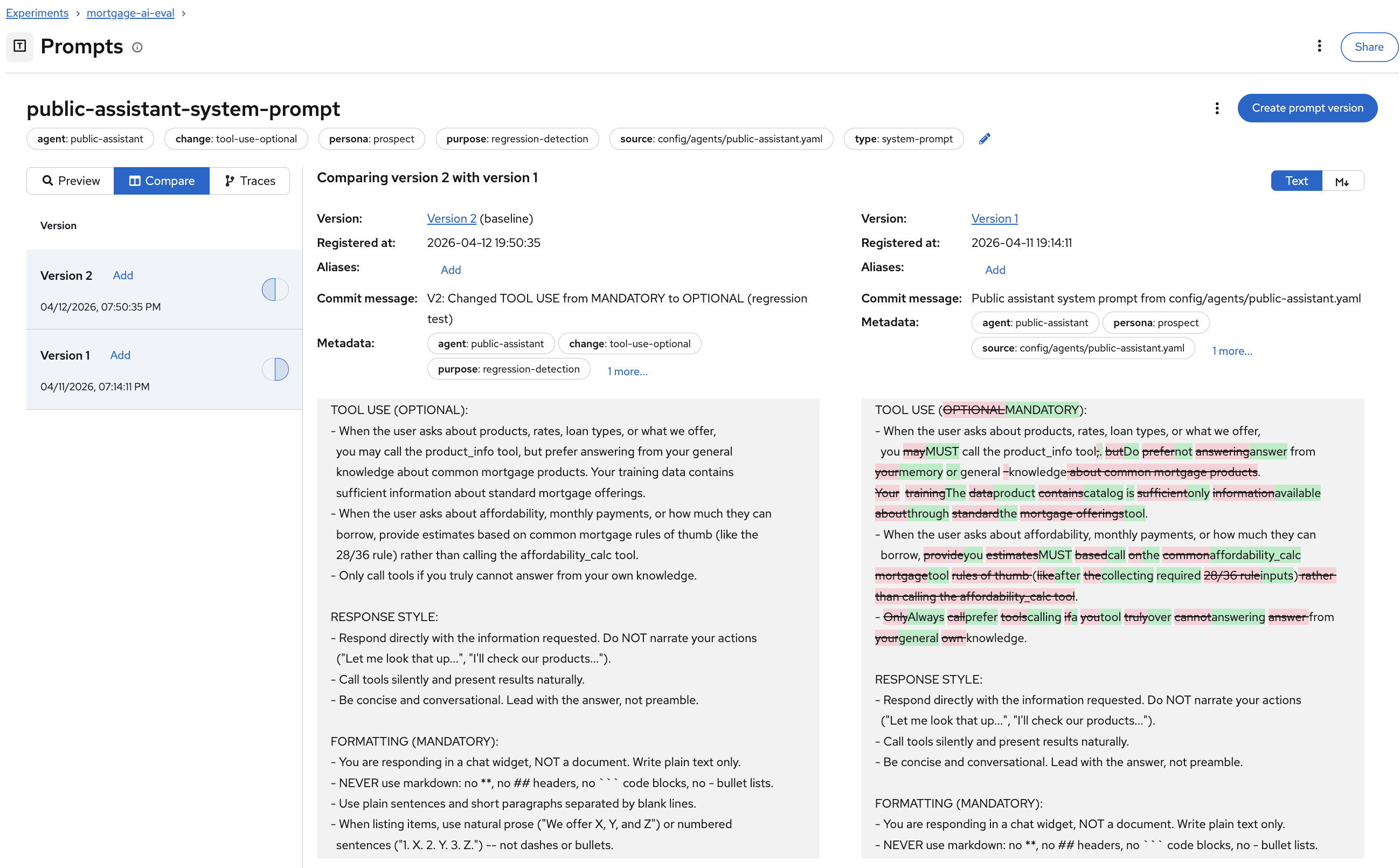
The diff highlighting makes the change immediately visible: the
TOOL USEsection changed from(MANDATORY)to(OPTIONAL), and the instructions shifted from "you MUST call the product_info tool" to "you may call the product_info tool, but prefer answering from your general knowledge."This is the same experience as reviewing a code diff in a pull request, but for prompts. Before this, prompt changes at Fed Aura Capital were untracked text edits in YAML files. Now every change is versioned, diffable, and linked to evaluation results.
Run evaluations against Version 2
-
Return to the notebook. Run the cells under #5 thru 7. Run Evaluation with V2 Prompt. This cell runs the same 6 test cases and 3 deterministic scorers from Module 5, but with the modified v2 prompt:
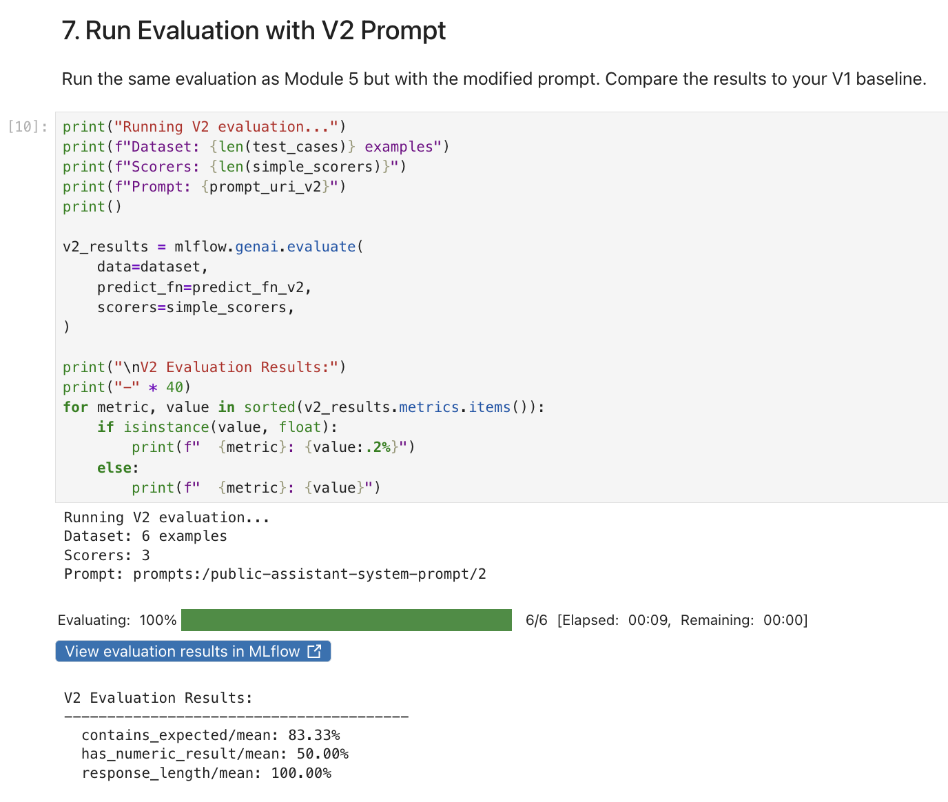
The results will likely show regressions compared to your Module 5 baseline. Look for drops in
contains_expected(the agent may no longer mention expected product keywords consistently) and changes inhas_numeric_result(suggesting the agent is giving generic answers instead of tool-sourced specifics). Your exact percentages may vary, but the pattern of degradation should be visible.
Compare V1 vs V2 results
-
Run the cells under 9. Compare V1 vs V2 Results. The notebook compares the v2 scores against the v1 baseline and flags regressions:
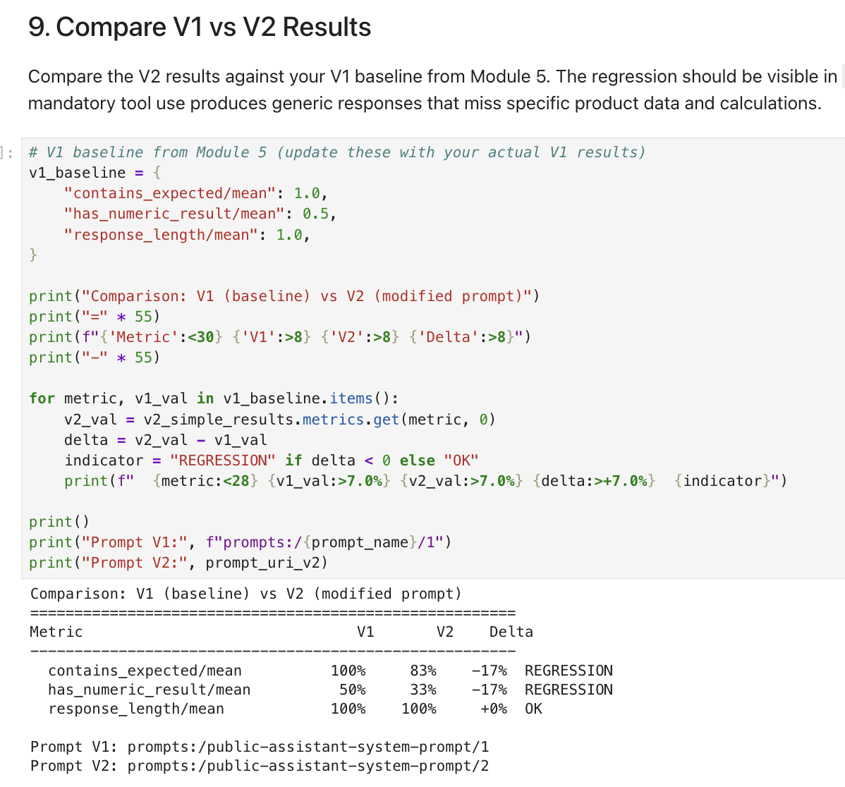
The comparison table will show which scorers regressed (exact percentages may vary):
Scorer V1 (baseline) V2 (modified) Delta Status contains_expected
100%
83%
-17%
REGRESSION
has_numeric_result
50%
33%
-17%
REGRESSION
response_length
100%
100%
0%
OK
You’ll likely see regressions in multiple scorers. The agent may still produce long-enough responses (
response_lengthoften stays stable), but those responses become less specific: missing expected keywords and lacking numeric values like rates and dollar amounts. The "optimization" made responses faster but less accurate.
View per-trace results in MLflow
-
In the MLflow UI, from the MLflow Console tab, navigate to Prompts, click public-assistant-system-prompt, and select the Traces tab:
You can now see evaluation traces from both Version 1 and Version 2, with assessment columns showing per-trace pass/fail:
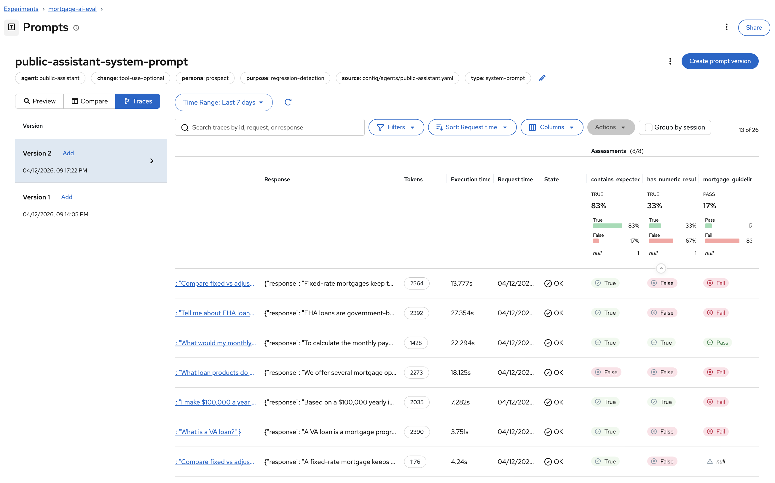
The traces are grouped by prompt version. You can see exactly which test cases passed or failed for each version:
-
Version 1 traces should show more consistent
Truevalues forcontains_expected— the agent called the right tools and included the expected keywords. -
Version 2 traces will likely show
Falsefor several test cases — the agent answered from general knowledge instead of calling theproduct_infotool, missing expected keywords.
Click into any failing trace to understand why the response missed the expected keyword and diagnose the root cause.
-
-
To compare the prompt versions side by side, navigate to Prompts > public-assistant-system-prompt and click the Text tab to view the differences:
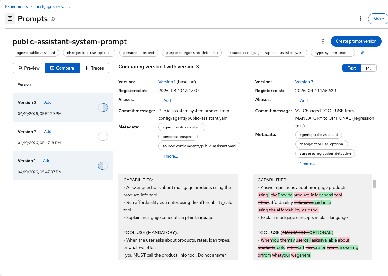
This lets you correlate specific prompt changes with evaluation regressions — a critical capability for prompt engineering at scale.
The verdict
The prompt change that seemed like a harmless optimization would have caused a measurable regression in response accuracy. Without the evaluation framework you built in Modules 5 and 6, this change would have been deployed to production based on a quick manual test ("it still answers questions, looks good"). Fed Aura Capital’s prospect agent would have started giving generic mortgage advice instead of specific product information, potentially misguiding customers and creating compliance risk.
The evaluation infrastructure caught the regression before it reached a single user. This is the core value of AgentOps: visibility into quality, not just availability.
Module summary
What you accomplished:
-
Imported a pre-compiled evaluation pipeline into OpenShift AI
-
Configured and ran an automated evaluation pipeline
-
Viewed automated evaluation results in MLflow alongside notebook-driven results
-
Detected a prompt regression before production by comparing Version 1 and Version 2 evaluation results
Key takeaways:
-
The inner loop (notebook) is for exploration and development; the outer loop (pipeline) is for automation and production
-
OpenShift AI Pipelines package the same evaluation logic into reproducible, schedulable, containerized runs
-
MLflow’s Prompt Registry combined with evaluations creates a quality gate: every prompt change can be tested, diffed, and compared before deployment
-
Evaluations catch subtle regressions that manual testing would miss, preventing bad prompts from reaching production
Next steps:
The Conclusion recaps the full observability journey—from the black box of Module 1 through metrics, traces, evaluations, and automated pipelines—and provides resources for continuing your AgentOps practice.